
Terrestrial carbon cycle parameter estimation - PowerPoint PPT Presentation
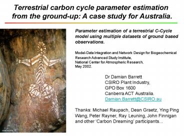
Title:
Terrestrial carbon cycle parameter estimation
Description:
from the ground-up: A case study for Australia. ... Climate data: BoM 0.25o Monthly max/min T(oC) (1950 - 2000) & Monthly rainfall(mm) (1890 - 2000) ... – PowerPoint PPT presentation
Number of Views:75
Avg rating:3.0/5.0
Title: Terrestrial carbon cycle parameter estimation
1
Terrestrial carbon cycle parameter estimation
from the ground-up A case study for Australia.
- Parameter estimation of a terrestrial C-Cycle
model using multiple datasets of ground based
observations. - Model-Data Integration and Network Design for
Biogeochemical Research Advanced Study Institute,
- National Center for Atmospheric Research,
- May 2002.
- Dr Damian Barrett
- CSIRO Plant Industry,
- GPO Box 1600
- Canberra ACT Australia.
- Damian.Barrett_at_CSIRO.au
- Thanks Michael Raupach, Dean Graetz, Ying Ping
Wang, Peter Rayner, Ray Leuning, John Finnigan
and other Carbon Dreaming participants...
2
Topics
- Background Motivations for developing yet
another terrestrial BGC model of the C-cycle. - Forward Model Conservation equations,
parameters, state variables, forcing functions,
and driver data. - Parameter estimation Recast the forward model
as a steady state model, multiple observation
datasets, search algorithm (GAs) and parameter
covariance matrix - Output Parameter estimates (turnover time of C
in soil and litter pools, depth profiles of soil
C efflux, light use efficiency of NPP).
3
Science Motivations 1 Reducing uncertainty in
carbon cycle
- Large uncertainties in the global C-cycle
particularly with terrestrial biogeochemistry,
particularly below ground processes. - Limited capability to observe below-ground
dynamics, fluxes and transformations of carbon. - Depth distribution of turnover time of C in
soil? - Depth distribution of soil C flux?
- Limited observations very patchy disparate
data - Limited process understanding
- Some processes are well understood
(photosynthesis d13C discrimination,
decomposition of litter and soil organic matter).
- Other processes are poorly understood
(C-allocation among plant tissues, T sensitivity
of humus decomposition, d13C discrimination of
decomposition)
4
Science Motivations 2 Approach in a nutshell
- An application of the parameter estimation
problem - using a forward model of NEE of C (VAST)
- multiple datasets of observations of plant
production and pool sizes to constrain parameters
in VAST. - Approach is distinct from Data Assimilation
- are not estimating initial conditions, updating
model state variables in time nor estimating
time dependent control parameters - are estimating steady state model parameters (ie
no time- or space-dependency in parameters) - We use algebraic scaling functions in the
forward model to introduce time- and
space-dependency in parameters
5
Scene setting Australia and North America
- Statistics Australia N. America
(Conterminous USA) - Land area (km2) 7.6 x 10⁶ 24.2 x 10⁶ (9.2 x
106 km2) - MAR 479 mm 630 mm
- Evaporation 437 mm 301 mm
- Runoff 50 mm 329 mm
- onset of agriculture 1860 1750
- Australia is characterized by high year-year
climate variability, high vapor pressure
deficits, highly weathered soils, high
biodiversity and an evergreen vegetation evolved
in isolation and adapted to these conditions
6
VAST1.1 Forward Model schematic diagram
- A linear compartmental model of C-dynamics of
the terrestrial biosphere - Linear dependence of qk and Pn on parameters.
- 10 pools
- Plant Production Light Use Efficiency approach
- Mortality and Decomposition modeled as
first-order kinetics. - Forced T, P, NDVI, fn,fs.
- 3 classes of parameters
- 12 Partitioning
- 10 Timescale
- Additional process e, r
Littermass
Biomass
Soil-C
7
VAST1.1 Forward Model
- VAST1.1 Input C-flux Light Use Efficiency model
- Mass conservation equations a system of 10
coupled first-order ODE.
8
VAST1.1 Forcing data
- Data
- Climate data BoM 0.25o Monthly max/min T(oC)
(1950 - 2000) Monthly rainfall(mm) (1890 -
2000) - NASA PAL 8km-10day NDVI Noise Filtered (Lovell
Graetz) re-georef (Barrett) (1981 - 2000) - NASA Langely SRB Monthly Shortwave down net
radiation (1983 - 1991) - Digital Atlas of Australian soils
Interpretation (McKenzie and Hook 1992) depth,
ksat. - Digital Atlas of Australian historic vegetation
Pre-European growth form of tallest stratum and
FPC.
9
VAST1.0 Multiple observations dataset
VAST 1.0 Observation Dataset 183 obs NPP
105 obs above ground biomass 94 obs fine
littermass 346 obs soil C 55 obs soil
bulk density From 174 published
studies. Available http//www-eosdis.ornl.gov
10
VAST Multiple observation datasets
interpretation
- Observation sites vegetation is minimally
disturbed - where the return period of stand replacing
disturbance is longer than the recovery period of
vegetation to maximum biomass. - Assume vegetation is at steady-state
- ie when averaged over space and time, the rate
of change of C-mass in any pool is zero (where C
influx into the biosphere C efflux from
biosphere). - Criteria to meet steady state assumption
- Authors description of overstorey vegetation
was equivalent with AUSLIG 1788 Historical
Australian Vegetation Classification - Age sequence oldest age vegetation used
- Multiple sites at a single lat/long data were
averaged among sites. - Only data from published literature was used
- (Quality control peer review)
- Only geo-referenced data used (lat/long)
11
VAST Observation datasets in climate space
AS
Savannahs
TF
- Open circles depict individual grid cells of
continental raster in climate space. - Colored circles show location of observations in
climate space. - NPP, Biomass and Littermass observations are
biased towards higher rainfall/productivity sites - Bias in the landscape (more productive sites)
- Soil observations are more representatively
distributed
NPP
qL qW
qF
Soil C
12
VAST Parameter estimation weighted least
squares
- Aim Estimate a by minimising the objective
function, O(a), given y, x y, - where
- y vector of observations for multiple datasets
(ie. the VAST 1.0 Obs Dataset) - y(.) corresponding vector of model predictions
(based on steady state equations) - x vector of forcing variables (climate,
radiation, NDVI) - a vector of model parameters
- Cy-1 is inverse of the error covariance matrix
(a symmetric weighting matrix containing
information on measurement error and correlations
among measurement errors). - where measurement errors are gaussian,
uncorrelated and errors constant variance (Cii
are equal Cij 0) Ordinary least squares - where Cii are not equal Cij 0 Weighted
least squares. - where Cii are not equal Cij ? 0 Generalised
least squares. - Multiple constraints case need to deal with
observations of unequal magnitude consequently
have unequal variances. - VAST1.1 we assume that measurement errors are
independent and gaussian and that the error
variances are equal to the sample variances for
each dataset.
13
VAST Specification of steady state model
- Since observations are from minimally
disturbed sites (ie. are assumed to represent
steady state conditions) we need to express the
conservation equations in steady state form. - Recalling that at steady state
- Re-arrange conservation equations steady-state
form - Where fk is the fraction of NPP which has passed
through pools upstream of qk.
14
VAST Specification of inverse model
- fk in VAST1.1 are
- Subject to
15
VAST Uncertainty in estimated parameters
- The uncertainty in parameters is given by the
parameter covariance matrix - Cb sy JT J-1
- where J is the Jacobian the matrix of model
derivatives with respect to parameters - The Jacobian is of dimensions n rows x p columns
(n Total Number of observations and p No. of
parameters) - Each element of the Jacobian is
- sy is the residual sum of squares
- sy y y(x a)T y y(x a) / (n p)
16
Parameter estimation using multiple datasets
- Equations in each y must share at least some
parameters in common - otherwise there is no mutual constraint imposed
by the multiple datasets (off diagonal elements
of JT J 0) - This is equivalent to independent parameter
estimates - Shared parameters between equations must be on
an equivalent SCALE - eg. Photosynthesis models at leaf and canopy
scales. - leaf scale Jmax e- transport processes in
chloroplast - canopy scale Jmax a statistical average over a
pop. - observations used to constrain the canopy model
cannot constrain estimates of the leaf scale
parameter (unless we have a way of disaggregating
the large scale information among the population
leaves).
17
Parameter estimation using multiple datasets
(continued)
- Highly correlated datasets add little information
to constrain parameter estimates - eg. Do N concentration datasets provide a
further constraint on C fluxes? - Due to conserved CN ratios in terrestrial
pools, C N data are highly correlated - Therefore including N data does not necessarily
add much new information to more tightly
constrain parameters. - In practice, Cy may be very difficult to specify
- particularly for multiple datasets where
information on error correlation between datasets
is unavailable.
18
Search method Genetic algorithms
- a type of stochastic search technique that is
particularly useful in optimisation where... - the region of the global minimum of O occupies a
small fraction of parameter space - parameter space is rough (numerous local minima)
- parameter space is discontinuous (jacobian is
unavailable) - Example shows the evolution of a solution to
the global minimum of a particularly difficult
function - Start with a random selection of population
members which are solutions to the problem and
evolves the population towards the global minimum
within 90 trials - Note
- local minima are not retained in the population
if other fitter members are found - even though the global minimum is found in lt 90
trials, mutation maintains diversity in the
search of parameter space
1
global minimum
60
90
19
Genetic algorithms a Primer
- Population is made up of a set of Chromosomes
(a set of parameters) comprising Genes (1
per parameter). - Each parameter value (gene) is encoded into a
binary string. - Crossover operator generates offspring from
mating parent chromosomes. - Mutation operator creates new genes
stochastically. - Selection Operator selects chromosomes based on
a Fitness function. - GAs generate solutions to problems by evolving
the population over time and selecting for fitter
solutions. They increase the average fitness of
a population of model solutions by exploiting
prior knowledge of parameter values retained in
the population. - For difficult objective functions Can use monte
carlo approaches to obtain estimates of parameter
uncertainties. (not done here)
mutation
crossover
selection
20
VAST Turnover time of soil C pools
- Estimated turnover time of C as a function of
soil depth (/- 1s) corrected for temperature and
moisture effects on decomposition - In situ turnover time at any time and place is
modified by climate, soil moisture content of the
soil and vegetation type. - Faster turnover of carbon in surface soil.
- Turnover time of C not significantly different
between 20 50 cm and 50 100 cm depths. - Increasing turnover time with depth reflects
decreasing decomposition rate, due to less labile
C, lower nutrient or oxygen availability,
increasing physical protection of C by higher
soil clay contents,
21
VAST Depth profiles of soil carbon flux
Tall productive forests
Open Woodlands
Arid shrublands
- Plots show realizations of the fraction of soil
C-flux originating from fine and coarse litter
pools and from different soil horizons for each
of the 3 vegetation types. - More than 89 of total soil C-flux originates
from lt 20cm depth (gt98 lt 50cm) - Largest source of C flux from soil is fine
litter - Model is relatively insensitive to uncertainty
in the estimated turnover time (predicted soil
respiration in 50 - 100 cm horizon has low
uncertainty).
22
Summary points
- To integrate inventory data, remote sensing, flux
station and atmospheric CO2 data for parameter
estimation we need to consider the following - We need a comprehensive set of forward models to
predict system state - predict fluxes f(NPP, stores, )
- predict fluxes f(near surface CO2, u, )
- predict radiance measures f(LAI, Fn, )
- predict atmospheric CO2 f(fluxes,
atmospheric transport, ) - We need the forward models to share common
parameters - otherwise no benefit obtained using multiple
constraints approach - Need to address issues of scale in order to
relate data obtained on different time and space
scales - eg the need to relate near surface CO2 to
atmospheric CO2 in order to combine eddy flux
and atmospheric CO2 datasets
23
Summary points continued
- We need an objective means for specifying the
network design (ie. a quantitative means of
identifying the types and locations of
measurements) - How do you decide whos network is better?
- network design is an optimization problem!
- so its possible to include in the objective
function a cost term for new observations - Is it better to generate extensive datasets of
cheap and uncertain observations over the scale
of interest, than few expensive accurate
observations? - We need analysis of the information content of
different types of datasets - because adding new datasets may not lead to
further constraint on model parameters if - new data are highly correlated with existing
data - if by adding new data we also add new model
equations having new unknown parameters (just
shifts the problem of insufficient information to
one of estimation of new parameters).
Recommended
CrystalGraphics Presentations


