Nyquist Stability Criterion

1
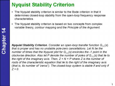
Nyquist Stability Criterion

• The Nyquist stability criterion is similar to the
  Bode criterion in that it determines closed-loop
  stability from the open-loop frequency response
  characteristics.
• The Nyquist stability criterion is based on two
  concepts from complex variable theory, contour
  mapping and the Principle of the Argument.

Nyquist Stability Criterion. Consider an
open-loop transfer function GOL(s) that is proper
and has no unstable pole-zero cancellations. Let
N be the number of times that the Nyquist plot
for GOL(s) encircles the -1 point in the
clockwise direction. Also let P denote the number
of poles of GOL(s) that lie to the right of the
imaginary axis. Then, Z N P where Z is the
number of roots of the characteristic equation
that lie to the right of the imaginary axis (that
is, its number of zeros). The closed-loop
system is stable if and only if Z 0.
2
Some important properties of the Nyquist
stability criterion are

• It provides a necessary and sufficient condition
  for closed-loop stability based on the open-loop
  transfer function.
• The reason the -1 point is so important can be
  deduced from the characteristic equation, 1
  GOL(s) 0. This equation can also be written as
  GOL(s) -1, which implies that AROL 1 and
  , as noted earlier. The -1 point
  is referred to as the critical point.
• Most process control problems are open-loop
  stable. For these situations, P 0 and thus Z
  N. Consequently, the closed-loop system is
  unstable if the Nyquist plot for GOL(s) encircles
  the -1 point, one or more times.
• A negative value of N indicates that the -1 point
  is encircled in the opposite direction
  (counter-clockwise). This situation implies that
  each countercurrent encirclement can stabilize
  one unstable pole of the open-loop system.

3

• Unlike the Bode stability criterion, the Nyquist
  stability criterion is applicable to open-loop
  unstable processes.
• Unlike the Bode stability criterion, the Nyquist
  stability criterion can be applied when multiple
  values of or occur (cf. Fig. 14.3).

Example 14.6 Evaluate the stability of the
closed-loop system in Fig. 14.1 for
(the time constants and delay have units of
minutes) Gv 2, Gm 0.25, Gc
Kc Obtain ?c and Kcu from a Bode plot. Let Kc
1.5Kcu and draw the Nyquist plot for the
resulting open-loop system.
4
Solution The Bode plot for GOL and Kc 1 is
shown in Figure 14.7. For ?c 1.69 rad/min, ?OL
-180 and AROL 0.235. For Kc 1, AROL ARG
and Kcu can be calculated from Eq. 14-10. Thus,
Kcu 1/0.235 4.25. Setting Kc 1.5Kcu gives
Kc 6.38.
Figure 14.7 Bode plot for Example 14.6, Kc 1.
5
Figure 14.8 Nyquist plot for Example 14.6, Kc
1.5Kcu 6.38.
6
Gain and Phase Margins
Let ARc be the value of the open-loop amplitude
ratio at the critical frequency . Gain margin
GM is defined as
Phase margin PM is defined as

• The phase margin also provides a measure of
  relative stability.
• In particular, it indicates how much additional
  time delay can be included in the feedback loop
  before instability will occur.
• Denote the additional time delay as .
• For a time delay of , the phase angle
  is .

7
Figure 14.9 Gain and phase margins in Bode plot.
8
or
where the factor converts PM from
degrees to radians.

• The specification of phase and gain margins
  requires a compromise between performance and
  robustness.
• In general, large values of GM and PM correspond
  to sluggish closed-loop responses, while smaller
  values result in less sluggish, more oscillatory
  responses.

Guideline. In general, a well-tuned controller
should have a gain margin between 1.7 and 4.0 and
a phase margin between 30 and 45.
9
Figure 14.10 Gain and phase margins on a Nyquist
plot.
10
Recognize that these ranges are approximate and
that it may not be possible to choose PI or PID
controller settings that result in specified GM
and PM values.
Example 14.7 For the FOPTD model of Example 14.6,
calculate the PID controller settings for the two
tuning relations in Table 12.6

• Ziegler-Nichols
• Tyreus-Luyben

Assume that the two PID controllers are
implemented in the parallel form with a
derivative filter (a 0.1). Plot the open-loop
Bode diagram and determine the gain and phase
margins for each controller.
11
Figure 14.11 Comparison of GOL Bode plots for
Example 14.7.
12
For the Tyreus-Luyben settings, determine the
maximum increase in the time delay
that can occur while still maintaining
closed-loop stability. Solution From Example
14.6, the ultimate gain is Kcu 4.25 and the
ultimate period is Pu
. Therefore, the PID controllers have the
following settings
13
The open-loop transfer function is
Figure 14.11 shows the frequency response of GOL
for the two controllers. The gain and phase
margins can be determined by inspection of the
Bode diagram or by using the MATLAB command,
margin.
14
The Tyreus-Luyben controller settings are more
conservative owing to the larger gain and phase
margins. The value of is calculated
from Eq. (14-14) and the information in the above
table
Thus, time delay can increase by as much as
70 and still maintain closed-loop stability.
15
Figure 14.12 Nyquist plot where the gain and
phase margins are misleading.