
The l chromosome PowerPoint PPT Presentation
1 / 32
Title: The l chromosome
1
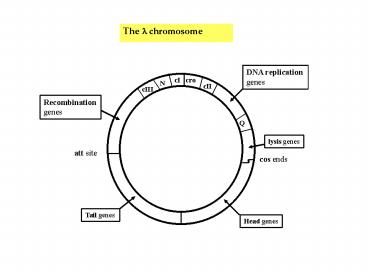
The l chromosome
DNA replication genes
cI
cro
N
cII
cIII
Recombination genes
Q
lysis genes
att site
cos ends
Tail genes
Head genes
2
patterns of gene expression
N, cro genes ON
very early
N, cro, Recomb, DNA rep genes ON
early
late
lysogeny
lysis
int, cI genes ON
lysis, head, tail genes ON
3
discussion of
Arkin A, Ross J, McAdams HH (1998) Stochastic
kinetic analysis of developmental pathway
bifurcation in phage l-infected Escherichia coli
cells, Genetics 149 1633-1648.
4
Fig 1
5
Fig 2
6
(No Transcript)
7
(No Transcript)
8
(No Transcript)
9
(No Transcript)
10
(No Transcript)
11
Fig 3
12
Fig 5
Fig 4
13
Gillespie Algorithm for stochastic chemical
kinetic simulations
P(t, m)dt probability at time t that the
next reaction will occur within (t t, t t
dt) and will be reaction m.
dt
t
time
t
(tt)
P(t, m) P(t)P(m) P(m) am /ao P(t)
aotexp(-aot)
0
1
am/ ao
a m -1/ ao
Ref Gillespie DT (1977) J. Phys. Chem. 81 2340.
14
Gilliespie program available here
http//www.sbw-sbml.org/sbw/software/index.html (y
ou first have to install SBW)
15
http//www.sbw-sbml.org/sbw/software/index.html
16
You can also download my FORTRAN program source
code (written years ago) from http//biopathways.
bu.edu/BE700/Links.html
17
1 A ? B 2 B ? A a1
c1XA a2 c2XB
Note for a reaction of the type
2R ? products one should use
a cXR(XR-1)/2
How to relate deterministic simula- ions with
stochastic simulations?
18
Assignment 2 Using the parameters that give
bistability in Assignment 1,
carry out a corresponding stochastic
(Gillespie) simulation
of the same network and show how the system
switches from one
steady state branch to the other.
Deterministic reaction rates
3
4
E
v1 k1EY/(Km1Y) k1bAY/(Km1bY)
A
v2 k2X/(Km2X)
1
Y
X
v3 k3X ko
v4 k4E
2
Note you must expand all enzymatic reaction
steps into elementary steps (to be discussed in
class).
A sample parameter set is ko0.0001, k30.04,
k40.1, k20.4, Km20.001, k1k1b1.5,
Km1Km1b0.01, (XY)total0.7
19
Tutorial on the (Gillespie) stochastic
simulation will be given.
Tutorial on bistability (Assignment 1)
Review/introduction of basic concepts used in
dynamical systems theory (phase portrait,
trajectories, stability) - done on whiteboard
20
QUALITATIVE NETWORK ANALYSIS
The purpose of this section is to define what a
qualitative network (qNET) is, and to show that
we can already generate some meaningful
conclusions about the stability of a network
despite the lack of pre- cise information on the
rate expressions and kinetic parameters. We will
also talk about some commonly occurring switching
mechanisms in biochemical systems.
Qualitative Networks (qNETs)
We begin by assuming that the system can be
described by a set of ordinary differential
equations shown in Eqn. 1. X is a vector of n
state variables (such as chemical concentrations
or enzyme activities) and F is n-vector of
functions of the state variables these functions
are usually nonlinear.
(1)
To determine the connectivity or topology of the
network, we imagine doing an experiment in which
we perturb the system from a reference state
(call this Xo ). An ideal reference state would
be a state in which all of the variables are not
changing (i.e. a steady state) but this not
required strictly in our discussion below. If x
represents the deviation (or perturbation) from
Xo , the time evolution of this perturbation
is given by Eqn..2. We refer to this equation as
the linearized system.
(2)
The network topology is revealed by the signs of
the mijs. Qualitative information such as
one species activating, inhibiting or
influencing another species can now be defined
as follows
21
The graphical representations of these
qualitative interactions are shown on the
right-most column above. At this point we simply
define a qualitative network (qNET) as a set of
nodes (the Xis) and a set of directed edges (the
qualitative interactions above). Note that each
edge connects a pair of nodes which are not
ne- cessarily different.
Example 1. Consider the linear pathway shown on
the left. Assume that step 1 represents a
constant rate of production of species X1 .
Also assume that all steps have mass action
kinetics. What is the corresponding qNET
diagram? See if you can arrive at the qNET
diagram shown on the right.
m11
m22
m33
X1
X2
X3
m21
m32
mechanism
qNET
22
qNET graph
Cycle strength
graph
Xi
1-cycle C(i) mii
Xi
Xj
2-cycle C(ij) mijmji
Xi
Xj
3-cycle C(ijk) mijmjkmki
Xk
23
an example
dX/dt k1 k2X dY/dt k2X k3Y
1
2
3
X
Y
qNET graph
P(l) l2 a1l a2 0 where a1 (-m11)
(-m22) a2 (-m11)(-m22)
24
Network topology and stability
You have learned earlier in this course how to
find the eigenvalues of the matrix M associated
with the linearized system. If each eigenvalue l
has a negative real part, then we know that the
system is locally stable the system is unstable
if there exists at least one l that has a
positive real part. At least in many cases,
local stability analysis could also predict
stability of the full nonlinear system. We now
want to show that only cycles in the qNET
diagram affect the local stability of the system.
Taking the qNET diagram in the previous page
(page) as a quick example, the edges associated
with m21 and m32 will not affect local
stability only the 1-cycles associated with m11,
m22, and m33 affect stability. To show this
claim, consider the characteristic polynomial
P(l) for an n-dimensional system (Eqn. 3).
P(l) det(lI-M) ln a1ln-1
a2 ln-2 an-1l an 0 where a1
?i -C1(i) a2 ?i,j -C1(i)-C1(j)
?jk -C2(j,k) a3 ?i,j,k -C1(i)-C1(j)-C1
(k) ?i,jk -C1(i)-C2(j,k) ?ijkC3(i,j,k)
... where C1(i) mii (1-cycles)
C2(jk) mjkmkj (2-cycles) C3(ijk)
mijmjkmki (3-cycles) ...
(3)
We refer to Ck as a k-cycle because it represents
a closed loop with k edges in the qNET diagram.
Since this notation is not quite standard, a
detailed example is given next.
25
eigenvalues are functions of cycles only
example (n2) P(l)
l2 a1l a2 0 where
a1 (-m11) (-m22) -C(1) -C(2) a2
(-m11)(-m22)(-m12m21) -C(1) -C(2)
-C(12)
26
Example 2. This examples shows how the
coefficients of the characteristic polynomial
P(l) are expressed in terms of k-cycles.
The mijs are the elements of the matrix M.
The coefficients are as follows
a1 (-m11) (-m22)
(-m33) -C1(1) -C1(2) -C1(3)
a2 (-m12m21)
(-m11)(-m22) (-m11)(-m33) (-m22)(-m33)
-C2(1,2) -C1(1)-C1(2) -C1(1)-C1(3)
-C1(2)-C1(3) a3 (-m13m32m21)
(-m21m12)(-m33) (-m11)(-m22)(-m33)
-C3(1,3,2) -C2(1,2)-C1(3)
-C1(1)-C1(2)-C1(3)
Next, we want to express network stability in
terms of the strengths of the k-cycles which
simply means the absolute value Ck. The
Routh-Hurwitz Theorem is a convenient one to use.
Refer to Clarke (1980).
27
First, it is necessary to define the Hurwitz
determinants, Di. Consider the array whose
elements are the coefficients of P(l) (see Eqn.
3)
a1 a3 a5 a7 1 a2 a4 a6 0
a1 a3 a5
The Hurwitz determinants are D1 a1
D2 a1a2 - a3 D3 a3D2 a1(a1a4-a5)
, etc.
Routh-Hurwitz Theorem. The number of eigenvalues
li with Re li gt 0 equals the sum of the number of
changes of sign in the sequences 1, D1,
D3, D5, and 1, D2, D4, D6, .
Example 3. The network given in Example 1 has
the following Hurwitz determinants D1 a1 gt
0 (since all the C1s are negative), D2
a1a2 - a3 and D3 a3D2 (since D4 D5 0).
Note that a3 gt 0. It looks like D2 can
change sign but it really doesnt. Do the
algebra and show that
D2 gt 0, and hence D3 gt 0. As expected, the
Routh-Hurwitz theorem therefore predicts
that the network in Example 1 is
always stable.
A very good exercise is to determine all the qNET
diagrams and their corresponding linear stability
for systems with two independent variables. The
result is shown in Fig. 1. Marginally stable
(MS) means that one eigenvalue is 0 but the other
is negative.
28
S C(3) m33
D C(12) m12 m21
T C(123) m21 m13 m32
sufficient instability conditions
1 S gt 0
29
S m33
D m12 m21
T m12 m23 m31
sufficient instability conditions
1 S gt 0
2 T lt 0
30
S m33
D m12 m21
T m12 m23 m31
sufficient instability conditions
1 S gt 0
2 T lt 0
3 SD lt T when T gt 0
31
Topology
Fig. 1
qNETs
U unstable
S stable
?
X
Y
MS marginally stable
?
? undecided
?
?
X
Y
?
?
?
X
Y
32
The reason why Fig. 1 is provided here is to give
an explicit example of how the topology and the
qualitative interaction already allows one to
infer the local stability of the network. This
kind of diagrams also answer ques- tions such as
What are additional interactions (or additional
species) that stabilize or destabilize a
network?. The arrows in Fig. 1 show what
additional interactions preserve the stability of
the network all other additional interactions
destabilize the system. The cases marked with
? are cases in which, indeed, the values of the
rate parameters will matter. These are very
interesting cases since there could be parameters
that switch the system from a stable to an
unstable state. See if you can give examples of
such networks.
Recommended
