Ch 10: An Introduction to Numerical Methods in Fortran 90 programs

1
Ch 10 An Introduction to Numerical Methods in
Fortran 90 programs

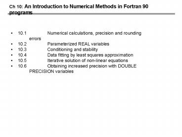
• 10.1 Numerical calculations, precision and
  rounding errors
• 10.2 Parameterized REAL variables
• 10.3 Conditioning and stability
• 10.4 Data fitting by least squares approximation
• 10.5 Iterative solution of non-linear equations
• 10.6 Obtaining increased precision with DOUBLE
  PRECISION variables

2

• FORTRAN 90 is useful for programming solutions to
  scientific programs. This is the subject of
  Numerical Methods.
• 10.1 Recall types
• INTEGER (e.g. numbers -109,, 109)
• REAL (e.g. numbers .d1d2d710/-e where e
  0,,38 i.e. exponent RANGE -38,38)
• As an example (HYPOTHETICAL) we consider
• REAL /- .d1d2d3d4 10/-e , where
• e 0,1,,9
• d1 1,2,3,..,9 EXP. RANGE -9,9
• d2,d3,d4 0,1,2,3,,9.

3
Figure 10.1 Number storage on the decimal
floating-point computer e.g. External
value Internal representation 37.5 0.3750
102 123.456 0.1235103 .12345678912345 0.12
35100 9876543210.1234 cannot be represented
exponent is 10 0.0000012345678 0.123410-
5 0.9999999999999 0.1101 0.0000000000375 ca
nnot be represented exponent is 10
4

• 9876543210.1234 .98771010 cannot be stored
  with HYPOTHETICAL REAL because e 10 gt 9. This
  is called overflow.
• Similarly, 0.0000000000375 .375 10-10, e -10
  lt -9. This is called underflow.
• Now, we will use HYPOTHETICAL REAL
• Examples of how computer arithmetic is done
  using registers
• e.g. a 11/9 .1222 101 (stored in memory)
• b 1/3 .3333 100 (stored in memory)

5
0.1222 101 0.0333 3 101 0.1555 3 101 (in
registers) 0.1555 101 (in
memory) Observe In exact arithmetic 11/9 1/3
11/9 3/9 14/9 .1556 101. So, we have
error 0.0001 101
6

• EXAMPLE WITH ADDING REAL NO.S OF DIFFERENT
  MAGNITUDES
• Consider now the result of a slightly longer
  calculation in which the five numbers 4 (0.4000
  101), 0.0004 (0.4 10-3), 0.0004, 0.0004 and
  0.0004 are added together. Since arithmetic on
  computers always involves only two operands at
  each stage, the steps are as follows
• 0.4000 101 0.0000 4 101 0.4000 4 101 (in
  registers)
• 0.4000 101 (in memory)
• (2) 0.4000 101 0.0000 4 101 0.4000 4 101
  (in registers)
• 0.4000 101 (in memory)
• etc.
• Observe exact result 4.002 .4002 101
  error
• 0.0002 101 i.e. 4th digit of fraction.

7

• Now consider what would have happened if the
  addition had been carried out in the reverse
  order
• 0.00040.00040.00040.00044 (INCREASING ORDER)
• 0.400010-3 0.400010-3 0.800010-3 (in
  registers)
• 0.800010-3 (in memory)
• (2) 0.800010-3 0.400010-3 1.200010-3 (in
  registers)
• 0.1200 010-2 (in registers)
• 0.120010-2 (in memory)
• (3) 0.120010-2 0.0400 010-2 0.160010-2 (in
  registers)
• 0.160010-2 (in memory)
• (4) 0.0001 6101 0.4000101 0.4001 6101 (in
  registers)
• 0.4002101 (in memory)

8
EXAMPLE OF SUBTRACTING 2 NO.S OF ALMOST SAME
MAGNITUDE 5/17 12/41 1/697 0.2941100 -
0.2927100 0.0014100 (in registers)
0.140010-2 (in memory) EXACTLY 5/17 12/41 is
equal to 1/697, or 0.1435 10-2
9
10.2 PARAMETRIZED REAL VARIABLES Working with
fixed REAL e.g. fraction of 4 digits and
exponents -9,,9 We see that may give errors in
the 4th or 3rd digit. This is not satisfactory
e.g. if we want all 4 digits to be
correct. Similarly, with our computers which
have fractions of 7 digits and exponents 0,
/-1, /-2,.,/-38 We may have only 5 correct
digits (because 6th, 7th digits have errors) just
in doing a subtraction.
10
FORTRAN 90 allows us to choose REAL types with
more precision. This is called parameterized
REAL and uses REAL(KIND ) e.g. REAL a, b
! This is default i.e. same REAL c, d ! as
e.g. KIND1 OR 2,. REAL, DIMENSION(10) x, y
REAL p(20), q(40), r(60) REAL(KIND4)
e, f REAL(KIND1) g, h REAL(KIND4),
DIMENSION(10) u, v REAL(KIND2) s(8),
t(5)
11
We can find the default type by e.g. j
KIND(x) e.g. REAL(KIND3) x REAL
y INTEGER i, j i KIND(x) j
KIND(y) Will give i3 and jdefault. We can
also omit keyword KIND REAL(4)
e,f REAL(1) g,h REAL(4), DIMENSION
u,v REAL(2) s(8), t(5)
12

• Observe
• KIND 1,2,3,4 etc. for REAL mean that the
  fraction has e.g. 7,14,21,28 digits and exponent
  range -30,30, etc.
• How many digits of fraction and what range for
  exponent are for a KIND depends on the
  computer.
• e.g. on one computer KIND 2 may be 14 digits
  of fraction and -100,100 exponent range and on
  another computer KIND 2 may be 6 digits of
  fraction and -30,30 exponent range.
• So, for portability we have e.g.
• (a)REAL(KINDSELECTED_REAL_KIND(P8, R30)) m
• (b)REAL(KINDSELECTED_REAL_KIND(P6, R30)) n

13

• Where p 8 minimum no. of digits of fraction,
  R 30 MINIMUM RANGE -30,30
• Most computers have
• SINGLE-PRECISION e.g. 6 digits of fraction and
  -40,40 exponent range
• DOUBLE-PRECISION e.g. 14 digits of fraction and
  
• -90,90 exponent range
• So, e.g. (b) is exactly the standard REAL type
  on a computer with 6 digits of fraction and
  -40,40 exponent range i.e. single-precision.
• But, (a) will be a double-precision because p 8
  gt 6 and
• p lt 13 and R 30 lt 90.

14
(4) Regardless of the computer the program with
(a) and (b) does not need to be changed. We can
define KIND INTEGER, PARAMETER real_8_30
SELECTED_REAL_KIND(P8, R30) ... REAL
(KINDreal_8_30) x, y, z
15

• Example
• Figure 10.2 shows the results of calculating the
  value of the following expression for different
  values of n.
• Figure 10.2 A comparison of the effect of
  different precisions
• Six digits of precision Fourteen
  digits of precision
• n Result Time
  (s) Result Time(s)
• 1.000 01 0.07 0.999 999
  999 999 98 0.10
• 2000000 0.985 693 13.66 0.999 999
  999 999 78 18.93
• 2500000 0.999 439 17.06 0.999 999
  999 999 80 23.72
• Note Time(s) is the execution time in seconds.

16
Real constants with KIND -103.4_7 ! Real of
kind type 7 3.14_high ! Real of kind type
high 4.0E7_2 ! Real of kind type 2 2.7 !
Default real (processor-dependent kind
type) INTEGER, PARAMETER real_8
SELECTED_REAL_KIND(P8) Chooses the default
value for exponent range R.
17
10.3 Conditioning And Stability

• A problem is well-conditioned if small changes
  in its input
• Parameters produce small changes in the output.
  If the
• opposite happens then the problem is
  ILL-conditioned.
• Examples of ill-conditioned problems
• (I)A quadratic equation roots
• (X 1)2 10-6 OR X2 2X (1 10-6)
  0
• roots P1 0.999 , P2 1.0001
• CHANGE Input parameter (coefficient) then the
  problem
• becomes
• (X 1)2 10-2 OR X2 2X (1 10-2) 0
  
• roots P1 0.9 and P2 1.1

18

• Small change in input parameter(i.e.change in
  constant coefficient)
• (1 10 6) ( 1 10 2) 10 2 10 6
  .01 .000001 .009999
• 
  0.01
• produces a large change in root P2 1.001 1.1
  .099 0.1
• REMARKS
• (1) In general the problem of calculating the
  roots of polynomials
• is ill-conditioned in terms of the
  polynomial coefficients
• (2) This ill-conditioning happens even if the
  method for
• calculating the roots produces no errors
  itself
• (3) The conclusion is that calculating the
  roots on computers even
• if the method is from an exact formula
  will produce errors if
• the coefficients are rounded off when
  entered to the computer
• e.g. if REAL has 2 digits then coefficient 0.999
  999 gt .10 E1 ( store in memory)
• 
  

19

• (4)Should we not solve(by computers)
  ill-conditioned problems(?)
• we should ! But we must increase the
  precision of REAL to
• double-precision in our program and the
  results (e.g. roots) will
• be accurate only in single-precision
  digits.
• (II) Another example of an ill-conditioned
  problem is the pair of
• simultaneous equations
• x y 10
• 1.002x y 0 solution x
  5000 y 5010
• Now if by some round-off of the
  coefficients had an error e.g.
• x y 10
• 1.001x y 0 solution x
  10000 y 10010

20

• So an error .001 in one of the coefficients
  produces an error
• (in x) -5000
• (in y) 5000. This problem is extremely
  ill-conditioned!
• .Now we look at errors in the numerical methods
  (or algorithms)
• A num. method is stable if the answer (output) is
  approximately
• the exact mathematical answer to the problem
  solved. A num.
• method is unstable if the answer it gives is for
  a problem different
• from the input (problem)

21

• Examples
• (I) Calculate e 5 with power series
• FROM calculus e x 1 x/1! x2/2! x3/3!
  .. AND if we
• truncate after the n-th term the error (in the
  truncation, not in round-off!)
• i.e. error En e x (1 x/1! x2/2!
  x3/3! (1)nxn/n!)
• is bounded En lt xne t/n!
• (truncation error)
• Where t is some number 0 lt t lt x
• e.g.
• for x 5 and n 25 the truncation error
• E25 lt 525 e t/25! lt 525/25! 210 8

22

• We use the program (to computee-5 in
  simple-precision i.e. 6
• 
  or 7 digits accuracy)
• PROGRAM exponential_unstable
• IMPLICIT NONE
• REAL x 5.0 , ans 0.0 , term 1.0
• INTEGER i
• PRINT (T5, i , T14 , TERMi , T29,
  SUMi)
• DO i 1, 25 !(1 x/1! x2/2!
  x3/3! (1)nxn/n! for n 25)
• ans ansterm
• PRINT ( I5 , 2X , 2E15.6 ) i ,
  term, ans
• term term( x)/REAL(i)
• END DO
• END PROGRAM exponential_unstable

23

• Figure 10.3 Results produced by using an
  unstable algorithm to calculate e-5
• TERMi( ( - 1)i Xi / i!)
  SUMi (ans)
• 
  
• 1 0.100000E 01
  0.100000E 01
• 14 -0.196033E 00
  -0.455547E 01
• 15 0.700119E 01
  0.244571E 01
• 24 -0.461122E 07
  0.673834E 02
• 25 0.960671E 07
  0.673844E 02
• BUT the correct answer (up to 6 digits of
  accuracy) is
• 0.673 79510-2. So, the method is unstable
  (because it alternately
• Subtracts the new term from the partial result

24

• REMEDY Find a stable algorithm (which does not
  use
• subtraction)
• NOTE ex (ex)1 (1 x/1! x2/2! x3/3!
  )1
• e.g. Sn 1 x/1! x2/2! x3/3! xn/n!
• The error (truncation) after n terms is En lt
  xnet/n! (1)
• for some t 0 lt t lt x
• since En ex (1 x/1! x2/2! x3/3!
  xn/n!) then
• truncation error in ex is En/ex(ex En)
  ..(2)
• (This is easy to check from calculus )
• For ( x 5 , n 25 ) using (1) we get
• E25 lt 2.9106 AND using (2) we get
• (truncation error for ex) lt 1.31010

25

• PROGRAM exponential_stable
• IMPLICIT NONE
• REAL x 5.0, r_and 0.0, term 1.0
• INTEGER i
• PRINT ( T5 , i, T14, TERMi ,T29,
  SUMi)
• DO i 1 , 25
• r_ans r_ans term ! 1 x/1!
  x2/2! x3/3! x25/n!
• PRINT(I5 , 2X, 2E15.7), I, term,
  1.0/r_ans
• term termx/FLOAT(i)
• END DO
• END PROGRAM exponential_stable

26

• Fig 10.4 Results produced by using a stable
  algorithm to calculate e-5
• TERMi
  SUMi
• 1 0.1000000E 01
  0.1000000E 01
• 24 0.4611219E 06
  0.6737946E 01
• 25 0.9606706E 07
  0.6737946E 02
• CORRECT answer 0.673799510-2
• 10.4 DATA FITING BY LEAST SQUARES
• Assume that we have a (set) table of data
  from experiments e.g and we want to pass a line
  as near to the data as possible. If we know that
  the data satisfy y ax b
• TABLE x y
• x1 y1
• 
  x2 y2
• 
  . .
• 
  xn yn

27

• We know (from p.69) that if we have n 2 pairs
  of data i.e.
• then there is one line connecting them (if x1 !
  x2)
• TABLE x y
• x1
  y1
• x2
  y2
• BUT if we have n gt 2, then it is not possible
  (expect special
• cases) for the line to connect the (x,y) points.
  Then we want a line
• to pass as near as possible

y
y7
y1
0 x1 x2..x7 x
28

• The problem of finding a line that passes as near
  as possible is
• solved by the least squares method which finds
  the a,b which
• make MINIMUM the sum axi b yi2
• From LINEAR ALGEBRA and CALCULUS we know that the
  
• Solution (assuming two xis at least are
  different) is
• 
  
• Note solve for a first and use it in b.

29

• For each (xi , yi) we call residual r(xi)
  axi b yi this states
• how closely the line y ax b passes through
  the point (xi , yi)
• e.g.
• 
  
• The residual sum
  
• gives the goodness of the fit. For best fit the
  residual sum

y
10r(x1)
0
x
x1 x2
x7
10r(x2)
30

• Example 10.1
• Assume that data of a wire are collected from an
  experiment
• figure 10.7 Experimental data from Youngs
  modulus experiment
• Weight
  Lengthlen
• 10
  39.967
• 12
  39.971
• 15
  39.979
• 17
  39.986
• 20
  39.993
• 22
  40.000
• 25
  40.007
• 28
  40.016
• 30
  40.022
• The diameter of
  wire(in inches) is 0.025

31

• Youngs modulus E stress / strain.
• E (f/A) /(
  ext/L)
• Where f is the force
• A is the cross-sectional area of
  circle
• ext is the extension due to weights
• L is the length of unstretched wire
• So, E (f L)/(A ext ) gt extension ext (
  fL)/(AE) kf where k L/(AE)
• Since ext len L len stretched wire
  length
• L
  unstretched wire length
• We find that the linear equation len L kf
  or len kf L
• must fit the experiment data. So we must
  calculate k and L as the
• a and b of the least squares method.Then we
  calculate the E
• From k L/(AE) gt E L/(A
  k)

32

• Solution
• MODULE constants
• IMPLICIT NONE   
• INTEGER,PARAMETER qSELECTED_REAL_KIND(P6,
  R30)  
• ! Define pi 
• REAL(KINDq), PARAMETER pi 3.1415926536_q
• ! Define the mass to weight conversion
  REAL(KINDq),PARAMETER g 386.0_q    
• ! Define the size of the largest problem set
  that can be processed
• INTEGER,PARAMETER max_dat100   
• END MODULE constants   

33

• PROGRAM youngs_modulus
• USE constants
• IMPLICIT NONE
• ! Input variables 
• REAL(KINDq), DIMENSION(max_dat) wt,len 
• REAL(KINDq) diam 
• INTEGER n_sets
• ! Other variables 
• REAL(KINDq) k,l,e  ! E in program is
  Youngs modulus
• INTEGER i   
• ! Read data 
• PRINT ,"How many sets of data?" 
• READ ,n_sets 

34

• ! End execution if too much or too little data 
  
• SELECT CASE (n_sets) 
• CASE (max_dat1 ) 
• PRINT ,"Too much data!" 
• PRINT ,"Maximum permitted is ",max_dat," data
  sets" 
• STOP 
• CASE ( 1) 
• PRINT ,"Not enough data!" 
• PRINT ,"There must be at least 2 data sets" 
  
• STOP 
• END SELECT
• PRINT ,"Type data in pairs weight (in lbs),
  length (in inches)" 

35

• DO i 1,n_sets 
• PRINT '("Data set ", I4, " ")',i 
• READ ,wt(i),len(i) 
• END DO
• PRINT ,"What is the diameter of the wire (in
  ins.)?" 
• READ ,diam   
• ! Convert mass to weight then wtf
• wt gwt   
• ! Calculate least squares fit 
• CALL least_squares_line(n_sets,wt,len,k,l)   
• ! Calculate Young's modulus 
• e (4.0_ql)/(pidiamdiamk)  ! E l /(pi
  (diam/2)(diam/2)k )

36

• ! Print results 
• PRINT '(//,5X,"The unstressed length of the wire
  is",  F7.3,"ins.")',l   
• PRINT '(5X,"Its Young''s modulus is ",E10.4,  
  " lbs/in/sec/sec"//)',e   
• END PROGRAM youngs_modulus      
• SUBROUTINE least_squares_line(n,x,y,a,b)   
• USE constants 
• IMPLICIT NONE   
• ! Dummy arguments 
• INTEGER,INTENT (IN) n 
• REAL(KINDq),DIMENSION(n),INTENT (IN) x,y 
• REAL(KINDq),INTENT (OUT) a,b   
• ! Local variables  REAL(KINDq)
  sum_x,sum_y,sum_xy,sum_x_sq   

37

• ! Calculate sums 
• sum_x SUM(x) 
• sum_y SUM(y) 
• sum_xy DOT_PRODUCT(x,y) ! This the sum of
  x(i)y(i), i1,..,n
• sum_x_sq DOT_PRODUCT(x,x)   
• ! Calculate coefficients of least squares fit
  line 
• a (sum_xsum_y n sum_xy )/( sum_x sum_x
  - nsum_x_sq) 
• b (sum_y - asum_x)/n   
• END SUBROUTINE least_squares_line

38

• NOTE The intrinsic function DOT_PRODUCT(VECTOR_A
  ,VECTOR_B) (see p.709) computes the dot product
  of 2 vectors e.g. vectors x(1n) , y(1n) then
  DOT_PRODUCT(x ,y) will compute
• RUN program youngs_modulus with input table
  Figure 10.7
• Figure10.8 Results produced by the program
  youngs_modulus
• How many sets of data?
• 9
• Type data in pairs weight (in lbs) , length (in
  ins.)
• Data set 9
• 30 40.022
• What is the diameter of the wire (in ins.)?
• 0.025
• The unstressed length of the wire is 39.938ins
• Its Youngs modulus is 0.1131E 11
  lbs/in/sec/sec

39

• 10.5 Iterative solution of nonlinear equations
• e.g. Linear equations
• The unknown(s) have exponent 1
• e.g. ax b c, where a!0, b, c are known
  constants and x is
• unknown gt closed form.
• Solution x (c b)/a
• Non-linear equations
• Given a non linear function of x (unknown) f(x)
  solve to find
• x f(x) 0
• e.g.
• 1) f(x) quadratic ax2 bx c 0 a, b,c
  known constants
• f(x) non-linear means there is at least one
  term in the expression
• of f(x) with exponent !0,1 or it is a
  function
• e.g. sinx , ex, logx etc

40

• 2) f(x) 63x3 183x2 97x 55 0
• non-linear e.g. exponents 3,2
• 3) f(x) x ex 0
• non-linear because it has terms e.g. ex (
  which is not x1)
• 4) f(x) x3 2sinx 0
• Using the computer we can approximate the
  solution (i.e. the
• zero or root) of the equation
  (non-linear) f(x) 0, for functions f(x) which
  are continuous e.g.
• The roots z1 ,z2 occur where the curve y f(x)
  intersects
• the x-axis (I.e the line y 0)

y
yf(x)
x
0
z1
z2
roots
41

• Since, the function f(x) is continuous (practical
  aspect we can
• draw it without lifting the pencil from the
  paper) the function
• f(x) gt 0 on the one side and f(x) lt 0 on the
  other side of the root
• (z1 or z2)
• e.g. if z2 4, z1 1 (in Fig 10.9, above )
  then f(x) lt 0, for 0 lt x lt 1 and f(x) gt 0 for 1 lt
  x lt 4 and f(x) lt 0, for 4 lt x lt 5
• Conclusion Given e.g. x ex 0 , f(x) 0
  with f(x) continuous,
• if we can find 2 points x0 lt x1 so that f(x0)
  f(x1) lt 0 then we
• know that there is at least one root of f(x) 0
  inside the interval
• (x0, x1) i.e f(z1) 0 and x0 lt z1 lt x1

42

• e.g.
• Here f(x0) gt 0 and f(x1) lt 0 gt f(x0) f(x1) lt
  0 gt root z1 lies
• in interval x0 , x1. we can obtain a computer
  method to
• approximate z1 as follows since the root z1 is
  in
• we bisect x0 , x1 i.e we take the middle
• Point x2 (x0x1)/2 and compute f(x2) and

y
f(x)gt0
yf(x)
0
x
x0
z1
x1
f(x)lt0
x0
x1
43

• if (I) f(x0)f(x2) lt 0 we continue (in the next
  step) with
• Else (II) f(x2)f(x1) lt 0 with
• Else (III) f(x2)0 and z1 x2.
• This method is iterative (i.e. it repeats some
  computations in each step or iteration) and
  we call it Bisection method.
• i-th step From step (i 1) we have
  
• because f(xi2)f(xi 1) lt 0. Let us call Ii
  1 xi 2 , xi 1 the
• interval which contains z1) at the i-th step
• We compute the mid-pt m xi 2 xi 1 /2

x0
x2
x2
x1
Xi-2
Xi-1
Z1
44

• We check If f(mi) 0 gt STOP (then z1 mi)
• If f(mi) f(xi 2) lt 0 then set xi m Ii
  xi 2 ,m xi 1 , xi
• ELSE SET Ii m, xi 1 xi 1 , xi
• We apply step-i for i1,..,n then length of
  interval
• In ½length(In-1) .. ½nlength(I0) (x1
  x0)/2n.
• If e.g. we want accuracy of approximation to the
  root z1 by e 10-7 ,
• then we must have length(In) lt 10-7. Then,
• z1 m z1 (xn xn 1)/2 lt length(In) lt
  10-7.

m
Z1
Xn-1
Xn
In
45

• Another check of accuracy of the approx. is
  f(Xn) lt e 10-7.
• Summary To approximate the root Z1 Xr (Xr is
  used in the book). We use the stopping tests or
  criteria e.g. with (tolerance for the error e
  10-7.
• The absolute value f(Xn) lt e
• OR
• - The length of In (i.e. (xn - xn 1) lt e )

46

• e.g. f(X) X2 3, X0,X1 1,2
• Signs of f(X), i.e. f(X) gt 0, f(X) lt 0.
• Iterations of Bisection method

Y
Z1
X
1
2
2
1
(12)/2 1.5
1.5
2
1.75
1.5
1.75
1.625
1.625
1.75
47

• Can we calculate the number of steps required to
  approximate the root Z1 with accuracy e 10-7
  YES.
• We need n iterations so that
• (X1 X0)/2n lt 10-7 gt (X1 X0)/10-7 lt 2n
• gtlog10(x1 x0) 7 lt log102n
• gtlog10(x1 x0) 7/log102 lt n
• e.g. here x1 2, x0 1 gt n must be such that
  
• log101 7/log102 lt n gt 9.97 lt n
• gt 10 lt n

48

• Other examples find roots on interval
• 
  x0 , x1
• f(x) x3 2sinx 0 ,
  ½ , 2
• f(x) 63x3 183x2 97x 55 0, -10 ,10
• x e x ,
  0,10
• create f(x)0 f(x) x - e-x 0, 0,10
• in all cases we must check
• f(x0)f(x1) lt 0
• Example 10.2. Write a program to find the root
  inside an interval
• i.e f(z1) f(xr) 0.
  We want to approximate
• xr. We only know that
  f(x0) f(x1) lt0.

Z1 or Xr
X0
X1
49

• Program input (information) data
• - external function f(x)
• - interval x0 , x1 call it left , right
• - tolerance (for error) e gt 0 tolerance
• - maximum number of iterations
  maximum_iterations
• Analysis We must program the i-th step inside a
  loop which
• terminates either if length(I_i) lt tolerance OR
  if reached
• maximum_iterations.
• Program structure plan
• 1) Read range (left and right), tolerance and
  maximum_iterations
• 2) Call subroutine bisect to find a root in the
  interval(left ,right)
• 3) If root found then
• 3.1 Print root
• otherwise
• 3.2 Print error message

50

• Subroutine bisect
• Real dummy arguments x1_start ,xr_start ,
  tolerance, zero,delta
• Integer dummy arguments max_iterations,
  num_bisecs, error
• Note that zero is the root, delta is the
  uncertainty in the root (it
• will not exceed tolerance), num_bisecs is the
  number of interval
• bisections taken and error is a status indicator
• 1 If x1_start and xr_start do not bracket a root
  then
• 1.1 Set error - 1 and return
• 2 Set x_left xl_start , x_right xr_start
• 3 Repeat max_iterations times
• 3.1 Calculate mid-point (x_mid) of interval
• 3.2 if (x_mid x_left)lt tolerance and then
  exit with
• zero x_mid, deltax_mid x_left and
  error 0 to indicate success.

51

• 3.3 Otherwise, determined which half interval
  the root lies in
• and set x_left and x_right appropriately
• 4 No root found so set error - 2 to indicate
  failure to converge
• quickly enough
• NOTE
• 1) (x_right x_mid) (x_mid x_left)
  length(I_i)
• 2) We evaluate f(x) only once in each iteration
  f(x_mid)
• The only slightly tricky step is step3.3 in which
  we determine
• which of the two intervals the roots lies
  in. We can expand
• this step as follows.

52

• 3.3.1 If f(x_left)f(x_mid) is less than 0 then
• 3.3.1.1 f(x_left) and f(x_mid)
  have opposite signs so
• set x_right to x_mid
  set f(x_right) f(x_mid)
• otherwise
• 3.3.1.2 f(x_left) and f(x_mid)
  have the same sign so set
• x_left to x_mid
  f(x_left) to f(x_mid)

53

• Solution
• MODULE constants
• IMPLICIT NONE
• ! Define a kind type q to have at least 6
  decimal digits
• ! and an exponent range form 1030 to
  10(-30)
• INTEGER, PARAMETER
• q SELECTED_REAL_KIND(P6, R30)
• END MODULE constants
• PROGRAM zero_find
• USE constants
• IMPLICIT NONE
• ! This program finds a root of the equation
  f(x)0 in a
• ! specified interval to within a specified
  tolerance of

54

• ! the true root, by using the bisection
  method
• ! Input variables
• REAL(KINDq), EXTERNAL f !MUST GIVE
  FUNCTION
• REAL(KINDq) left, right, tolerance
• INTEGER maximum_iterations
• ! Other variables
• REAL(KINDq) zero, delta
• INTEGER number_of_bisections, err
• ! Get range and tolerance information
• PRINT , "Give the bounding interval (two
  values)"
• READ , left, right

55

• PRINT , "Give the tolerance"
• READ , tolerance
• PRINT , "Give the maximum number of iterations
  
• 
  allowed"
• READ , maximum_iterations
• ! Calculate root by the bisection method
• CALL bisect(f, left, right, tolerance,
  maximum_iterations,
• zero, delta, number_of_bisections, err)
• ! Determine type of result

56

• SELECT CASE (err)
• CASE (0)
• PRINT , "The zero is ", zero, "- ",
  delta
• PRINT , "obtained after ",
  number_of_bisections,
• 
  " bisections"
• CASE (-1)
• PRINT , "The input is bad i.e. initial
  interv.
• Does not contain a root"
• CASE (-2)
• PRINT , "The maximum number of iterations
  
• has been exceeded"
• PRINT , "The x value being considered
  was ", zero
• END SELECT
• END PROGRAM zero_find

57

• SUBROUTINE bisect(f, xl_start, xr_start,
  tolerance,
• max_iterations,zero,
  delta, num_bisecs, error)
• USE constants
• IMPLICIT NONE
• ! This subroutine attempts to find a root
  in the interval
• ! xl_start to xr_start using the bisection
  method
• ! Dummy arguments
• REAL(KINDq), INTENT(IN) xl_start, xr_start,
  tolerance
• INTEGER, INTENT(IN) max_iterations
• REAL(KINDq), INTENT(OUT) zero, delta
• INTEGER, INTENT(OUT) num_bisecs, error

58

• ! Function used to define equation whose roots
  are required
• REAL(KINDq), EXTERNAL f
• ! Local variables
• REAL(KINDq) x_left, x_mid, x_right, v_left,
  
• v_mid, v_right
• ! Initialize the zero-bounding interval and the
  function
• ! values at the end points
• IF (xl_start lt xr_start) THEN
• x_left xl_start
• x_right xr_start
• ELSE
• x_left xr_start
• x_right xl_start

59

• END IF
• v_left f(x_left)
• v_right f(x_right)
• If(v_left . OR. v_right 0.0) Then error 0
  Return
• ! Validity check
• IF (v_left v_right gt 0.0 .OR. tolerance lt 0.0
  .OR.
• max_iterations lt 1) THEN
• error -1
• RETURN
• END IF

60

• DO num_bisecs 1, max_iterations
• delta 0.5 (x_right-x_left)
• x_mid x_left delta
• IF (delta lt tolerance) THEN
• ! Convergence criteria satisfied
• error 0
• zero x_mid
• RETURN
• END IF
• Note Compute f(X_mid) ONCE in each iteration.
• v_mid f(x_mid)

61

• 
  
• ! Remove the following print statement when the
  program
• ! has been thoroughly tested
• PRINT ("Iteration", I3, 4X, 3F12.6, " (",
  F10.6, ")"),
• num_bisecs, x_left, x_mid,
  x_right, v_mid
• 
  
• ! f(x_left)f(x_mid) lt0.0
• IF (v_left v_mid lt 0.0) THEN
• ! A root lies in the left half of the
  interval
• ! Contract the bounding interval to the
  left half
• x_right x_mid
• v_right v_mid
• ELSE ! f(x_mid)f(x_right) lt 0
• ! A root lies in the right half of the interval
• ! Contract the bounding interval to the right
  half

62

• x_left x_mid
• v_left v_mid
• END IF
• END DO
• ! The maximum number of iterations has been
  exceeded
• error -2
• zero x_mid
• END SUBROUTINE bisect
• FUNCTION f(x)
• USE constants
• IMPLICIT NONE
• ! Function type
• REAL(KINDq) f

63

• ! Dummy argument
• REAL(KINDq), INTENT(IN) x
• f x EXP(x)
• END FUNCTION f
• Note We are computing the root of f(x) x eX
  0
• OR eX -x.
• Note from calculus e.g. X0,X1 -10,0

Y
y -x
y ex
1
X
Root Zero
64

• Bisection program output
• Give the bounding interval (two values)
• -10, 0
• Give the tolerance
• 1E-5
• Give the maximum number of iterations allowed
• 100
• X_mid f(X-mid)
• Iteration 0 -10.000000 -5.000000 0.000000
  (-4.993262)
• Iteration 1 -5.000000 -2.500000 0.000000
  (-2.417915)
• Iteration 18 -0.567169 -0.567150 -0.567131
  (-0.000011)
• The zero is -0.5671406 - 9.5367432E-06
  (delta lt 10-5)
• obtained after 19 bisections

65

• SIGN (1, v_left) (see p.711) returns the sign
  i.e./- 1 of v_left.
• So, we use this instead of IF(v_leftv_mid) lt
  0.0
• We have IF(SIGN(1,v_left)SIGN(1,v_mid)) lt 0
• The reason for this is to avoid OVERFLOW which
  happens if
• v_leftv_mid gt 1030
• e.g. for v_left 1016, v_mid 1015