Calibration Methods

1
Calibration Methods

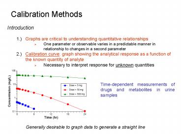
• Introduction
• 1.) Graphs are critical to understanding
  quantitative relationships
• One parameter or observable varies in a
  predictable manner in relationship to changes in
  a second parameter
• 2.) Calibration curve graph showing the
  analytical response as a function of the known
  quantity of analyte
• Necessary to interpret response for unknown
  quantities

Time-dependent measurements of drugs and
metabolites in urine samples
Generally desirable to graph data to generate a
straight line
2
Calibration Methods

• Finding the Best Straight Line
• 1.) Many analytical methods generate calibration
  curves that are linear or near linear in nature
• (i) Equation of Line
• where x independent variable
• y dependent variable
• m slope
• b
  y-intercept

3
Calibration Methods

• Finding the Best Straight Line
• 2.) Determining the Best fit to the Experimental
  Data
• (i) Method of Linear Least Squares is used to
  determine the best values for m (slope) and b
  (y-intercept) given a set of x and y values
• Minimize vertical deviation between points and
  line
• Use square of the deviations ? deviation
  irrespective of sign

4
Calibration Methods

• Finding the Best Straight Line
• 4.) Goodness of the Fit
• (i) R2 compares the sums of the variations
  for the y-values to the best-fit line relative to
  the variations to a horizontal line.
• R2 x 100 percent of the variation of the
  y-variable that is explained by the variation of
  the x-variable.
• A perfect fit has an R2 1 no relationship for
  R2 0

R2 based on these relative differences Summed for
each point
R20.5298
R20.9952
Very weak to no relationship
Strong direct relationship
53.0 of the y-variation is due to the
x-variation What is the other 47 caused by?
99.5 of the y-variation is due to the x-variation
5
Calibration Methods
Calibration Curve 1.) Calibration curve shows a
response of an analytical method to known
quantities of analyte

• Procedure
• Prepare known samples of analyte covering
  convenient range of concentrations.
• Measure the response of the analytical
  procedure.
• Subtract average response of blank (no analyte).
• Make graph of corrected response versus
  concentration.
• Determine best straight line.

6
Calibration Methods

• Calibration Curve
• 2.) Using a Calibration Curve
• Prefer calibration with a linear response
• - analytical signal proportional to the
  quantity of analyte
• Linear range
• - analyte concentration range over which
• the response is proportional to
• concentration
• Dynamic range
• - concentration range over which there
• is a measurable response to analyte

Additional analyte does not result in an increase
in response
7
Calibration Methods

• Calibration Curve
• 3.) Impact of Bad Data Points
• Identification of erroneous data point.
• - compare points to the best-fit line
• - compare value to duplicate measures
• Omit bad points if much larger than average
  ranges and not reproducible.
• - bad data points can skew the best-fit line
  and distort the accurate interpretation of data.

y0.091x 0.11 R20.99518
y0.16x 0.12 R20.53261
Remove bad point Improve fit and accuracy of
m and b
8
Calibration Methods

• Calibration Curve
• 4.) Determining Unknown Values from Calibration
  Curves
• (i) Knowing the values of m and b allow the
  value of x to be determined once the
  experimentally y value is known.
• (ii) Know the standard deviation of m b, the
  uncertainty of the determined x-value can also be
  calculated

9
Calibration Methods

• Calibration Curve
• 4.) Determining Unknown Values from Calibration
  Curves
• (iii) Example

The amount of protein in a sample is measured by
the samples absorbance of light at a given
wavelength. Using standards, a best fit line of
absorbance vs. mg protein gave the following
parameters m 0.01630 sm 0.00022 b
0.1040 sb 0.0026 An unknown sample has an
absorbance of 0.246 0.0059. What is the amount
of protein in the sample?
10
Calibration Methods

• Calibration Curve
• 5.) Limitations in a Calibration Curve
• (iv) Limited application of calibration curve to
  determine an unknown.
• - Limited to linear range of curve
• - Limited to range of experimentally
  determined response for known
• analyte concentrations

Uncertainty increases further from experimental
points
Unreliable determination of analyte concentration
11
Calibration Methods

• Calibration Curve
• 6.) Limitations in a Calibration Curve
• (v) Detection limit
• - smallest quantity of an analyte that is
  significantly different from the blank
• where s is standard deviation
• - need to correct for blank signal
• - minimum detectable concentration

Signal detection limit
Corrected signal
Detection limit
12
Calibration Methods

• Calibration Curve
• 6.) Limitations in a Calibration Curve
• (vi) Example
• Low concentrations of Ni-EDTA near the detection
  limit gave the following counts in a mass
  spectral measurement 175, 104, 164, 193, 131,
  189, 155, 133, 151, 176. Ten measurements of a
  blank had a mean of 45 counts. A sample
  containing 1.00 mM Ni-EDTA gave 1,797 counts.
  Estimate the detection limit for Ni-EDTA

13
Calibration Methods

• Standard Addition
• 1.) Protocol to Determine the Quantity of an
  Unknown
• (i) Known quantities of an analyte are added to
  the unknown
• - known and unknown are the same analyte
• - increase in analytical signal is related to
  the total quantity of the analyte
• - requires a linear response to analyte
• (ii) Very useful for complex mixtures
• - compensates for matrix effect ? change in
  analytical signal caused by
• anything else than the analyte of
  interest.
• (iii) Procedure
• (a) place known volume of unknown sample in
  multiple flasks

14
Calibration Methods

• Standard Addition
• 1.) Protocol to Determine the Quantity of an
  Unknown
• (iii) Procedure
• (b) add different (increasing) volume of known
  standard to each unknown sample
• (c) fill each flask to a constant, known volume

15
Calibration Methods

• Standard Addition
• 1.) Protocol to Determine the Quantity of an
  Unknown
• (iii) Procedure
• (d) Measure an analytical response for each
  sample
• - signal is directly proportional to analyte
  concentration

Standard addition equation
Total volume (V)
16
Calibration Methods

• Standard Addition
• 1.) Protocol to Determine the Quantity of an
  Unknown
• (iii) Procedure
• (f) Plot signals as a function of the added
  known analyte concentration and
• determine the best-fit line.

X-intercept (y0) yields which is
used to calculate from
17
Calibration Methods

• Standard Addition
• 1.) Protocol to Determine the Quantity of an
  Unknown
• (iii) Example

Tooth enamel consists mainly of the mineral
calcium hydroxyapatite, Ca10(PO4)6(OH)2. Trace
elements in teeth of archaeological specimens
provide anthropologists with clues about diet and
disease of ancient people. Students at Hamline
University measured strontium in enamel from
extracted wisdom teeth by atomic absorption
spectroscopy. Solutions with a constant total
volume of 10.0 mL contained 0.750 mg of dissolved
tooth enamel plus variable concentrations of
added Sr. Find the concentration of Sr.
18
Calibration Methods

• Internal Standards
• 1.) Known amount of a compound, different from
  analyte, added to the unknown.
• (i) Signal from unknown analyte is compared
  against signal from internal standard
• Relative signal intensity is proportional to
  concentration of unknown
• - Valuable for samples/instruments where
  response varies between runs
• - Calibration curves only accurate under
  conditions curve obtained
• - relative response between unknown and standard
  are constant
• Widely used in chromatography
• Useful if sample is lost prior to analysis

Area under curve proportional to concentration of
unknown (x) and standard (s)
19
Calibration Methods

• Internal Standards
• 1.) Example

• A solution containing 3.47 mM X (analyte) and
  1.72 mM S (standard) gave peak areas of 3,473 and
  10,222, respectively, in a chromatographic
  analysis. Then 1.00 mL of 8.47 mM S was added to
  5.00 mL of unknown X, and the mixture was diluted
  to 10.0 mL. The solution gave peak areas of 5,428
  and 4,431 for X and S, respectively
• Calculate the response factor for the analyte
• Find the concentration of S (mM) in the 10.0 mL
  of mixed solution.
• Find the concentration of X (mM) in the 10.0 mL
  of mixed solution.
• Find the concnetration of X in the original
  unknown.