
A recent study repeated Standing PowerPoint PPT Presentation
1 / 80
Title: A recent study repeated Standing
1
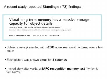
A recent study repeated Standings (73) findings
-
- Subjects were presented with 2500 novel real
world pictures, over a few hours - Each picture was shown once, for 3 seconds
- Immediately afterwards, a 2AFC recognition
memory test (which is familiar?)
2
(No Transcript)
3
- Conclusions
- High memory capacity
- High fidelity
4
Binary Synapses Slower Than Expected
- Work with Peter Latham
Amit Miller
Research Talk
Oct. 2008
5
Outline
- Quick review
- When its good
- When its bad
- Correlations in the noise
6
One shot, serial learning
The brain is doing serial learning with no
repetitions
7
One shot, serial learning
External stimulus clamp
neuronal activity
stimulus A
8
One shot, serial learning
External stimulus clamp
neuronal activity
stimulus A
Activity-dependent plasticity follows
9
One shot, serial learning
External stimulus clamp
neuronal activity
stimulus A
stimulus B
Activity-dependent plasticity follows
10
One shot, serial learning
External stimulus clamp
neuronal activity
stimulus A
stimulus B
stimulus C . . .
Activity-dependent plasticity follows
11
One shot, serial learning
External stimulus clamp
neuronal activity
stimulus A
stimulus B
New memories overwrite old memories memories get
degraded and decay
stimulus C . . .
Activity-dependent plasticity follows
12
Assumption discrete synapses only two
efficacies are allowed
Synapses are bound, and discrete
Strong (potentiated)
Strong (potentiated)
state switches
Weak (depressed)
Weak (depressed)
Fortunately,- we have many synapses (N of
them)- synapses are stochastic
13
The learning rule
- External stimuli dictate plasticity by randomly
choosing neurons - Plasticity is Hebbian
(neurons and synapses, under external stimulus)
Potentiation pre post f02
Depression pre post f0
f1 Indifferent otherwise
14
but synapses do not switch deterministically
- External stimuli only dictate candidates for
potentiation and depression - Actual state switches are performed
stochastically - Synapses are stochastic state machines
- State transitions are described by stochastic
matrices - Upon potentiation M
- Upon depression M-
15
Assumption synapses are i.i.d.
- Corollary I
- We can forget about neurons for now. Care only
for synapses - We have a large population N synapses of
variables
f fraction of synapses, candidates for
plasticity (sparseness) f fraction of
the candidate synapses, destined for potentiation
(balance) f - (1- f )
fraction of the candidate synapses, destined for
depression
16
Assumption synapses are i.i.d.
- Corollary II
- We focus on the distribution of synaptic states -
P(t) - over a large population of synapses - We use a Mean-Field approach, and derive
everything from the state distribution
17
What happens when we learn a new stimulus
Space of synapses
The synaptic state distribution is at equilibrium
18
What happens when we learn a new stimulus
Stimulus A
19
What happens when we learn a new stimulus
Stimulus A
20
What happens when we learn a new stimulus
Stimulus A
21
What happens when we learn a new stimulus
Potentiated (M) sub-population
Stimulus A
Depressed (M-) sub-population
22
What happens when we learn a new stimulus
Potentiated (M) sub-population
Stimulus A
Depressed (M-) sub-population
23
What happens when we learn a new stimulus
Potentiated (M) sub-population
Stimulus A
Depressed (M-) sub-population
24
What happens when we learn a new stimulus
Ideal Observer
25
Forgetting
Stimulus A
Stimulus B
26
Forgetting
Stimulus A
Stimulus B
27
Forgetting
Stimulus A
Stimulus B
Stimulus C
28
- Mean Signal
- S(t) w ? ( P(t) - Peq )
- Initial distribution
- P(0) M Peq
- Evolution in time Markov Chain
- P(t) Ht P(0)
Reference level - and - starting point
29
Markov Chain
- The stochastic matrix H describes the mean effect
of new memoriesH (1- f )I f f M
(1-f )M- - Corollaries
- P(t) converges to Peq
- The signal decays to zero
30
Memory lifetime
0
The width of the distributions is given by the
noise at equilibrium - seq
31
Summary
- Construct matrices
- Calculate the equilibrium distribution
- Calculate the initial distributions
- Iterate Markov Chain until stopping criterion
- Optimize w.r.t. to model parameters
32
Two main models
- The 2-State synapse (Binary synapse)
- The Multi-State synapse
33
The 2-State synapse
State transitions
- Simple
- Analytically solvable
- Exponential decay
34
- Fast learning means fast forgetting
- Tradeoff initial Signal-to-Noise vs. memory
lifetime
35
The Multi-State synapse
- The Cascade model Fusi, Drew, Abbott. Neuron,
2005 - Allow both strong initial S/N and long memory
lifetime - Power-law behavior
36
- A model may have n internal states
for n 8
Transition probabilities in/out of a state are
falling off exponentially For state of depth d,
xd
37
- A model may have n internal states
for n 8
38
(No Transcript)
39
(No Transcript)
40
Results
- Comparison of the Multi-State and 2-State synapses
41
Enhanced
Standard
Perfect balance f 1/2
42
Enhanced
Modified
Standard
f 0.9
43
Modified
Enhanced
Standard
N 109, f 0.01
44
Modified
Enhanced
Standard
N 109, f 0.01
45
Outline
- Quick review
- When its good
- When its bad
- Correlations in the noise
46
Eigenvalue decomposition of H
- And therefore
47
Finally
The signal is written as a sum of weighted
exponentials
S(t) ?k ßk exp(?k t)
w vk vkP(0)
, k ? 0 ßk w vk
vkP(0) wPeq 0 , k 0
48
n -1 exponentials
Last one to survive
49
At long times, a Multi-State model behaves as its
slowest exponential
S(t) ß1 exp(?1 t)
50
Memory lifetime depends on ß1 and ?1
?n-1 and ßn-1
ß1
Better
Worse
Binary model
51
Memory lifetime depends on ß1 and ?1
?n-1 and ßn-1
Multi-State ?
ß1
Binary model
52
Optimizing ß1 and ?1 for memory
lifetimeyields an optimal memory lifetimewhich
is independent of the number of states. Thus,
all models 2-State included are
equivalent. The only condition the eigenvalues
must be well separated
53
d
0
e ltlt d
54
Outline
- Quick review
- When its good
- When its bad
- Correlations in the noise
55
Its all about the Equilibrium Distribution
exponential fall-off in transition probabilities
sensitivity to the balance between potentiation
and depression
56
Standard model, x 1/2
57
- The noise is lower
- But the signal is hit much more badly
58
Solution 1 the Modified model
- fine-tune w.r.t. f
- Uniform distribution among negative/positive
states - Comes at a price
x 1- f
59
Enhanced
Modified
Standard
f 0.9
60
Solution 2 the Enhanced model
- Optimize both x and
- The constraint now is
x - goes very low, x approaches 1
- No exponential fall-off, transition probabilities
are of the same magnitude
61
Enhanced
Modified
Standard
f 0.9
62
Outline
- Quick review
- When its good
- When its bad
- Correlations in the noise
63
Dependence on the Signal-to-Noise ratio
- Memory lifetime is extracted by solving
- We assumed that synapses are i.i.d., hence
Noiseeq was proportional to the variance of a
single synapse - But, in reality, different synapses may share
pre- and post-synaptic neurons
64
Correlations 2nd order only
Pairs of synapses may co-vary their efficacy
depending on the learning rule
post
post
pre
pre
pre
post
post
Type 1
Type
3 Type 2
Type 4
pre
post/pre
pre/post
post
pre
65
- Nsynapses Mneurons x Kconnections
K in 1 .. M-1 - Random connectivity, every neurons making
exactly K pre- post-synaptic connections
66
Signal
Mean Signal
67
And the noise (at equilibrium)
68
- We use K 1500
- Still, M gtgt K
69
How to calculate the joint P(Ja,Jb)?
Peq is extracted from the transition matrix
(principal eigen vector)
- -
--
H n x n
70
Approximation
- Collapse all positive and negative states
together - We are interested in the net negative / positive
probability p(), p(-) - At equilibrium and not the convergence
towards equilibrium - Synaptic pairs, at equilibrium, still maintain
the same marginals
71
A necessary condition for equilibrium
Equal transition mass between the two sets of
states
H2 4 x 4
72
Some results
73
(No Transcript)
74
(No Transcript)
75
(No Transcript)
76
N 1010 synapses, f 0.1
77
N 1010 synapses, f 0.1
78
(No Transcript)
79
(No Transcript)
80
So
- Disclaimers
- I might be wrong
- Reasonable choice of K
- Reasonable learning rule
- Conclusions with a barrel of salt
- Multi-State synapses cant really deliver
- Strong initial S/N ? large covariance ? stronger
noise - You cant beat the trade-off
Recommended
