
V7 - Graph Layout of Cellular Networks PowerPoint PPT Presentation
1 / 34
Title: V7 - Graph Layout of Cellular Networks
1
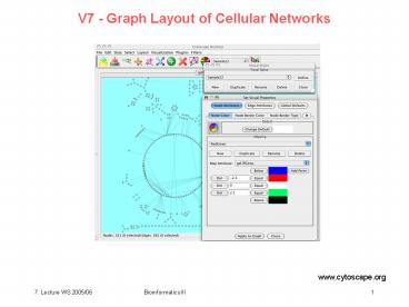
V7 - Graph Layout of Cellular Networks
www.cytoscape.org
2
Task visualize cellular interaction data
e.g. protein interaction data (undirected)
nodes proteins edges interactions metabo
lic pathways (directed) nodes
substances edges reactions regulatory
networks (directed) nodes transcription
factors regulated proteins edges regulatory
interaction co-localization (undirected) nodes
proteins edges co-localization
information homology (undirected/directed) node
s proteins edges sequence similarity (BLAST
score)
3
Graph layout algorithms
Graphs are often used to encapsulate the
relationship between items. Graph drawing
enables visualization of these relationships.
The usefulness of visualizations depends upon
whether the drawing is aesthetic. While there
are no strict criteria for aesthetic drawing, it
is generally agreed that such a drawing has -
minimal edge crossing, - emphasis of symmetry,
and - even spacing between vertices. Many
approaches have been proposed in the literature.
However, most useful operations for drawing
general graphs have been proved to be
NP-complete. 3 popular straight-edge drawing
algorithms are - the spring model and -
spring-electrical model Both work by minimizing
the energy of physical models of the graph. -
high-dimensional embedding method is quite
different.
documents.wolfram.com
4
Force-directed algorithm for graph layout
In 1984, Peter Eades proposed a graph layout
heuristic which is called the Spring Embedder''
algorithm. Edges are replaced by springs and
vertexes are replaced by rings that connect the
springs. A layout can be found by simulating the
dynamics of such a physical system. In a system
governed by physical forces, the system will
adopt a low-energy conformation. This method and
other methods, which involve similar simulations
to compute the layout, are called Force
Directed'' algorithms.
http//www.hpc.unm.edu/sunls/research/treelayout/
node1.html
5
Variant1 Spring model
The spring model assigns force between each pair
of nodes. When two nodes are too close together,
a repelling force comes into effect. When two
nodes are too far apart, they are subject to an
attractive force. This scenario can be
illustrated by linking the vertices with springs
- hence the name "spring model" (or "spring
embedding method"). This algorithm works by
adding springs to all edges and adding looser
springs to all vertex pairs that are not
adjacent. Thus, in 2D, the total energy of the
system is Here, xi and xj are the
coordinate vectors of nodes i and j, and xi -
xj is the Euclidean distance between them.
lij natural length of the spring between
vertex i and vertex j, lij can be chosen as the
graph distance between i and j. The parameters
kij R / lij2 are the strength of the springs,
where R is a parameter representing the strength
of the strings. V is the number of vertices.
documents.wolfram.com
6
Spring model
The layout of the graph vertices is calculated by
minimizing this energy function finding minima
where the derivative is lowest. The negative
derivative of the (scalar) energy is the
(vectorial) force One way to minimize the
energy function is by iteratively moving each of
the vertices along the direction of the spring
force until an approximate equilibrium is
reached. Multilevel techniques are used to
overcome local minima. The spring model works
well for problems like regular grid graphs, in
which it is possible to lay out the graph so that
physical distances between vertices are
proportional to the graph distances. One
disadvantage of the spring model it requires
knowing the graph distance between every pair of
vertices.
Why is the force the negative and not the
positive derivative?
documents.wolfram.com
7
Variant2 Spring-electrical model
The spring-electrical model uses two types of
forces. (1) The attractive force is restricted
to adjacent vertices and is proportional to the
physical distance between them. (2) The
electrical force is global and is inversely
proportional to the distance between nodes.
Overall, the energy to be minimized is
Here, C is a constant that regulates the
relative strength of the repulsive and attractive
forces, dij is the Euclidean distance between
nodes i and j, and K is the natural spring length.
documents.wolfram.com
8
Variant2 Spring-electrical model
When computing the force
The first term is repulsive and inversely
proportional to the square distance. This is
analogous to a repulsive Coulombic interaction
between two equally charged particles. As all
nodes repel eachother with a uniform force, the
nodes will equally spread over the available
space (except for boundary effects). The second
term is attractive and grows linearly with the
distance. This is analogous to a spring force
between connected (?) nodes that keeps them close
together.
documents.wolfram.com
9
Coulomb-Gesetz
- Das Coulomb-Gesetz wurde durch Henry Cavendish
(1731-1810), - J Priestley (1733 1804) und CA Coulomb
(1736 1806) in sorgfältigen Experimenten an
makroskopischen Objekten wie Magneten,
Glasfäden, geladenen Kugeln und Kleidung aus
Seide entdeckt. - Es gilt auf einer sehr weiten Größenskala
einschließlich Atomen, Molekülen und biologischen
Zellen.
Charles Coulomb
Henry Cavendish
Die Wechselwirkungsenergie u(r) zwischen 2
Ladungen q1 und q2 im Abstand r voneinander ist
im Vakuum
mit der Proportionalitätskonstante
10
Force-directed algorithm
Example showing graph optimization by
spring-electrical algorithm.
http//www.it.usyd.edu.au/aquigley/3dfade/
11
Force-directed algorithm
Because of the underlying analogy to a physical
system, the force directed graph layout methods
tend to meet various aesthetic standards, such as
- efficient space filling, - uniform edge
length (when equal weights and repulsions are
used) - symmetry and the - capability of
rendering the layout process with smooth
animation (visual continuity). Having these
nice features, the force directed graph layout
has become the work horse'' of layout
algorithms. A side-effect of this algorithm is
that vertices at the periphery tend to be closer
to each other than those in the center. Why? Not
so nice the initial random placement of nodes
and even very small changes of layout parameters
will lead to different representations.
http//www.hpc.unm.edu/sunls/research/treelayout/
node1.html
12
Scaling
Force directed layout methods commonly have
computational scaling problems. When there are
more than a few thousand vertexes in the graph,
the running time of the layout computation can
become unacceptable. This is caused by the fact
that in each step of the simulation, the
repulsive force between each pair of unconnected
vertexes needs to be computed, costing a running
time of O(0.5 ? V2 E). Here V is the number of
vertexes and E is the number of edges in the
graph. Multilevel techniques are used to
overcome local minima, and an octree data
structure is used to reduce the computational
complexity in some cases. With multilevel and
octree techniques, it is implemented very
efficiently with a complexity of about O(V log
V ). In general, the spring-electrical model
works well for most problems.
http//www.hpc.unm.edu/sunls/research/treelayout/
node1.html
13
H3
This system was developed between 1996 and 1998
by put picture Tamara Munzner to visualize large
data sets of Tamara Munzner ?100.000
nodes. Focusses on quasi-hierarchical graphs
that can be effectively visualized using a
spanning tree as the backbone of a layout
algorithm, e.g. E V to E 4
V. Spanning tree connected acyclic subgraph
that contains all the vertices of the original
graph, but does not have to include all the
links. Here cast building of a spanning tree as
a problem that must be solved at each node, by
selecting which of the incoming links to a node
would be the best one to use as the parent for
that node in the spanning tree. find a
minimum-weight spanning tree through a graph with
weighted edges, where domain-specific information
is used to compute the weights.
PhD thesis Tamara Munzner, chapter 3
14
H3
Constructing a spanning tree for
quasi-hierarchical web site. Top Left The
hyperlink structure of a simple hypothetical
site, as it would be reported by a web spider
starting at the top page. Nodes represent web
pages, and links represent hyperlinks. Although
the graph structure itself is determined by
hyperlinks, additional information about
hierarchical directory structure of the sites
files is encoded in the URLs. Top Row We build
up the graph incrementally, one link at a time.
Middle Row We continue adding nodes without
moving any of the old ones around. Bottom Row
When the animal/wombat.html page is added, the
label matching test shows that animal is a more
appropriate parent than /TOC.html, so the node
moves and the link between animal/wombat.html and
/TOC.html becomes a non-tree link. In the final
stage, note that bird/emu.html does not move when
the bird is added, even though the labels match,
because there is no hyperlink between them.
PhD thesis Tamara Munzner, chapter 3
15
H3
Constructing a spanning tree for
quasi-hierarchical function call graph. In this
simple hypothetical function call graph, nodes
represent functions, and links represent calls
from one function to another. The call graph is
computed by a static analysis of the program
text. The spanning tree is determined by run-time
profiling of the code so that the calling
procedure that is responsible for the most
execution time in the called procedure is the
parent. We show the layout incrementally as in
the figure before the parent of a node can
change when new information about a more
appropriate candidate emerges, and the small
multiples should be read row by row starting at
the top left
PhD thesis Tamara Munzner, chapter 3
16
where to place nodes?
The classic problem with tree layout in Euclidean
space is that the number of child nodes to place
grows exponentially at each level of the tree,
but the available room in which to place them
grows only polynomially. Specifically, the
circumference of a circle (2?r) or the area of a
sphere (4?r2) increases as a polynomial function
of its radius r. The usual approach to avoiding
collisions is to allocate less room to nodes
deeper in the tree than to ones near the root.
Disadvantage when using a fine zoom level one
can only see a small local neighborhood of any
leaf node, when using a coarse zoom level to see
the entire tree, the leaf nodes are too small to
see. Distortion-based visualization methods
strive to show detail within as much surrounding
context as possible in a given amount of screen
area. The H3 system uses hyperbolic geometry for
both layout and navigation.
PhD thesis Tamara Munzner, chapter 3
17
Hyperbolic geometry
Hyperbolic geometry is one of the non-Euclidean
geometries developed at the turn of the century.
Here it was used for two reasons (1) there is
an elegant way to draw a FocusContext view using
a known projection that maps the entire infinite
space into a finite drawing region. (2) one can
allocate the same amount of room for each of the
nodes in a tree while still avoiding collisions
because there is an exponential amount of room
available in hyperbolic space. Hyperbolic and
spherical geometry are the only two non-Euclidean
geometries that are homogeneous and have
isotropic distance metrics there is a uniform,
meaningful, and continuous concept of the
distance between two points. These geometries
are internally consistent despite the lack of
Euclids parallel postulate. In the spherical
case there are no parallel lines all great
circles intersect each other. In the hyperbolic
case there are many lines through a point that
are parallel to another line.
PhD thesis Tamara Munzner, chapter 3
18
Exponential room
In hyperbolic space, circumference and area
increase exponentially with respect to radius.
There is literally more room in hyperbolic space
than in Euclidean space, where these measures
increase polynomially. The circumference of a
hyperbolic circle increases exponentially with
respect to its radius the equation is 2p sinh r,
as opposed to the Euclidean equation 2pr.
Figure 3.3 shows a picture of the 2D
hyperbolic plane embedded into 3D Euclidean
space, intended to give an intuitive sense of
how much more room there is on a hyperbolic
plane than on a Euclidean plane.
PhD thesis Tamara Munzner, chapter 3
19
Exponential room
Most pictures of the 2D hyperbolic plane show one
of the traditional projective or conformal views
where projected features appear smaller on the
periphery. This picture instead shows a piece
of the 2D hyperbolic plane where true sizes are
not distorted, so the only way to display it in
3D Euclidean space is with overlapping folds.
PhD thesis Tamara Munzner, chapter 3
20
Models of hyperbolic space
PhD thesis Tamara Munzner, chapter 3
21
Visualization with H3
PhD thesis Tamara Munzner, chapter 3
22
Visualization with H3
PhD thesis Tamara Munzner, chapter 3
23
Aim analyze and visualize homologies between the
protein universe -) 50 genomes ? 145579
proteins ? 21 ? 109 BLASTP pairwise sequence
comparisons. Expect that fusion proteins
(Rosetta Stone proteins) will link proteins of
related function. Need to visualize extremely
large network! Develop stepwise scheme.
24
LGL
Stepwise scheme (1) separate original network
into connected sets (2) generate coordinates for
each node in each connected set (using
force-directed layout algorithm and a recipe for
the sequential lay out of nodes guided by a
minimum spanning tree of the network). (3)
integrate connected sets into one coordinate
system via a funnel process the connected sets
are sorted in descending size by the number of
vertices. The first connected set is placed at
the bottom of a potential funnel and other sets
are placed one at a time on the rim of the
potential funnel and allowed to fall towards the
bottom where they are frozen in space upon
collision with the previous sets. We concentrate
on step (2) in the following
Adai et al. J. Mol. Biol. 340, 179 (2004)
25
Minimum Spanning Tree
Given undirected graph G (V,E) where for each
edge (u,v) ? E exists a weight w(u,v) specifying
the cost to connect u and v. Find an acyclic
graph T ? E that connects all of the nodes and
whose total weight is minimized.
Popular algorithms by Kruskal and Prim. Both are
greedy algorithms making the best choice at the
moment. ? no guarantee to find the best global
solution
Cormen
26
Kruskals algorithm
Consider edges in sorted order by weight. The
arrow points to the edge under consideration at
each step.
Cormen
27
Kruskals algorithm (II)
Running time ? O(E log V)
Cormen
28
Intuitive description of LGL
Successive iterations of the layout. The MST
determines the oder of placement of the nodes.
The root node could be chosen randomly or based
on its centrality in the network (e.g. minimizing
the sum of distances to all other nodes). All
other nodes are assigned a level according to
their edge-based distance in the MST from the
root node. Level one vertices (red circles) are
placed randomly on a sphere around the root node
(black circle). The system is allowed to iterate
through time satisfying attractive and repulsive
forces until at rest. Level two nodes (blue
circles) are placed randomly on spheres directed
away from the current layout. Again, the system
is allowed to evolve through time till at rest.
This process is iterated for the entire graph.
Adai et al. J. Mol. Biol. 340, 179 (2004)
29
What is the role of fusion proteins?
A protein homology map summarizes the results of
billions of sequence comparisons by modeling the
proteins as vertices in a network, and the
statistically significant sequence similarities
as edges connecting the relevant proteins. In
this manner, proteins within a sequence family
(such as A, A', A?, and AB or B, B' and AB) are
all or mostly connected to each other, forming a
cluster in the map. Fusion proteins (such as AB)
serve to connect their component proteins'
families. The structure of the resulting map
reflects historic genetic events, such as gene
fusions, fissions, and duplications, which are
responsible for producing the modern-day genes.
The map simultaneously represents homology
relationships (edges), remote homologies
(proteins not directly connected but in the same
cluster), and non-homologous functional
relationships (adjacent clusters and clusters
linked by fusion proteins).
Adai et al. J. Mol. Biol. 340, 179 (2004)
30
LGL Algorithm for very large biological networks
The complete protein homology map. A layout of
the entire protein homology map a total of
11,516 connected sets containing 111,604 proteins
(vertices) with 1,912,684 edges. The largest
connected set is shown more clearly in the inset
and is enlarged further on the right side.
Adai et al. J. Mol. Biol. 340, 179 (2004)
31
Map of gene function
emerges from 21 billion gene sequence
comparisons. Proteins are drawn as points, with
lines connecting proteins with similar sequences,
and are arranged so that homologous proteins are
adjacent in the Figure. The size of each cluster
is proportional to the number of proteins in that
sequence family. Fusion proteins force their
component proteins' respective families to be
close together in the Figure, and thereby serve
to organize the proteins in the map according to
their functions. The resulting broad trends of
protein function are labeled, as are several of
the most extensive sequence families. AC
indicate specific regions that are magnified
later.
Only the greatest connected network component is
drawn, containing 30,727 proteins (vertices) and
1,206,654 significant sequence similarities
(edges), and representing 4 billion sequence
comparisons.
Adai et al. J. Mol. Biol. 340, 179 (2004)
32
Functionally related gene families form adjacent
clusters
Three examples illustrate spatial localization of
protein function in the map, specifically A,
the linkage of the tryptophan synthase ? family
to the functionally coupled but non-homologous ?
family by the yeast tryptophan synthase ?? fusion
protein, B, protein subunits of the pyruvate
synthase and alpha-ketoglutarate ferredexin
oxidoreductase complexes C, metabolic enzymes,
particularly those of acetyl CoA and amino acid
metabolism.
Adai et al. J. Mol. Biol. 340, 179 (2004)
33
Colocalization
Neighboring proteins tend to be in the same
cellular system. The tendency for proteins to
operate in the same cellular system, as defined
by the percentage of matching assignments into
the 18 COG database pathways, is plotted against
the spatial separation in multiples of a typical
cluster size. The functional similarity decays
exponentially with distance proportional to the
function e-0.26d where d is a typical cluster
diameter.
Adai et al. J. Mol. Biol. 340, 179 (2004)
34
Comparison with other layout maps
A comparison of LGL with map layouts produced by
other algorithms. The layout of the protein
homology map by LGL (A) is contrasted with the
layout of the same network by the spring-force
algorithm only, lacking the minimal spanning tree
calculation and iterative layout procedure (B),
and with the layout by the approach of
InterViewer (C). Interviewer collapses
equivalent nodes into single nodes, thereby
simplifying the graph, and is one of the few
available graph layout programs that scales to
such large networks. The layout from LGL reveals
more of the internal graph structure than the
other approaches tested.
Adai et al. J. Mol. Biol. 340, 179 (2004)
Recommended
