The%20Reaction%20module

1
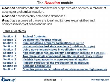
The Reaction module

• Reaction calculates the thermochemical properties
  of a species, a mixture of species or a chemical
  reaction.
• Reaction accesses only compound databases.
• Reaction assumes all gases are ideal and ignores
  expansivities and compressibilities of solids and
  liquids.

Table of contents
Section 1 Table of Contents Section 2 Opening
the Reaction module Section 3 Pure substance
property calculations (pure Cu) Section
4 Isothermal standard state reactions (oxidation
of copper) Section 5 Using non-standard states
in equilibrium reaction Section 6 Non-isothermal
non-equilibrium calculation (heating of pure
(Al)) Section 7 Two phase single component
equilibrium (ideal binary system) Section
8 Variable input amounts in non-isothermal
reaction Section 9 Pidgeon Process for the
Production of Magnesium Section 10 Aqueous
applications Section 11 Complex gases and
condensed substances under high pressure
1
2
The Reaction module
Click on Reaction in the main FactSage window.
2
3
Reactants window - entry of a species (pure Cu)
Add a Product
Reaction has two windows Reactants and Table
Add a Reactant
Reaction can only access compounds (not solutions)
Open
New Reaction
Entry of reactant species
All calculations shown here use the FACT compound
databases and are stored in FactSage - click on
File gt Directories gt Slide Show Examples
Compound databases available
Go to the Table window
3.1
4
Table window thermodynamic properties of a
species
Open
Save
New Reaction
Stop Calculation
Summary of the Reactants window
A multiple entry for T min, max and step. The
results also display the calculated transition
temperatures.
Return to the Reactants window
3.2
5
Determination of most stable phase by Gibbs
energy minimization
3.3
6
Simple isothermal standard state reaction
oxidation of copper
Entry of an isothermal standard state reaction
4 Cu O2 2 Cu2O
This example is stored in FactSage. Go to the
menu bar and click on File gt Directories gt
Slide Show Examples and select file 2.
Isothermal T throughout
Go to the Table window
Non standard states checkbox is not selected
4.1
7
Oxidation of copper at various temperatures
Entry Tmin300K, Tmax2000K and step300K. Note
the transition temperatures.
The equilibrium constant column appears for an
isothermal standard state reaction. DGº -RT lnK
. For the values of the gas constant R, click on
the Units menu.
4.2
8
Simple chemical equilibrium non standard state
oxidation of copper
aCu(s) X
PO2(g) P
Select non standard state
Standard state reaction PO2(g) 1.0 atmaCu(s)
1.0
5.1
9
Specifying an extensive property change to deal
with chemical equilibrium
For simple chemical equilibrium
and DG0 -RT ln Keq
when DG 0.
Table provides DG using
and

• For the last entry
• PO2(g) 10-12
• aCu(s) 1
• DG 0, equilibrium

5.2
10
Heating Al from 300 K to the temperature T
phase transition, Al(s) Al(l) (i.e. fusion) at
933.45 K DHfusion Tfusion DSfusion
28649.1J - 17938.1J 10711.0 J
The equilibrium constant is not displayed because
this is a non-isothermal non-equilibrium
calculation.
6.1
11
Heating Al creating the graphical display with
Figure
1. Click on the menu Figure and select Axes...
2. A dialog box opens and provides you with a
choice of axes for the figure.
Click on Refresh for the default settings
6.2
12
Heating Al graphical display of thermodynamic
properties
liquid
17.9 kJ
Point the mouse to read the coordinates of the
melting point.
solid
933 K
6.3
13
Computation of Cu liquidus in an ideal binary
system data entry
Equilibrium of the type Me(pure solid,T) Me
(liquid,a(Me) x(Me),T)
Cu(solid) Cu(liquid)
aCu(solid) 1, pure solid copper
aCu(liquid) X

• Selection of phases
• phases from the FACT database
• 2 compound databases are included in the Data
  Search but here only FACT data are selected.

7.1
14
Computation of Cu liquidus in an ideal solution
mixing databases
2. FACT and SGPS compound databases are selected
1. Click on the Data Search menu.
7.2
15
Computation of Cu liquidus in an ideal binary
system tabular and graphical output
Calculated activity of Cu(liquid) in equilibrium
(DG0) with pure Cu(solid) at various
temperatures T.
For an ideal solutionaCu(liquid) XCu(liquid)
Liquid
Liquidus line
Liquid Solid
The 2 specified variables, T and DG, are
highlighted.
Note When DG 0, the reaction must be
isothermal.
7.3
16
Variable input amounts in non-isothermal reaction
and autobalance feature

• The following example shows how a variable amount
  of a reactant can be used to simulate an excess
  of this substance, i.e. its appearance among both
  the reactants and the products.
• A simple combustion reaction
• CH4 ltAgt O2 CO2 2 H2O ltA-2gt O2
• The Alpha variable, ltAgt, is used to define the
  quantity of O2.

8.0
17
Combustion of CH4 in variable amount ltAlphagt O2
data entry
The reactants are at 298 K but the products are
at an unspecified T.
Variable quantity ltAlphagt
The phase of each species is specified.

• The reaction is non-isothermal (except when T
  298 K). Hence
• Keq will not appear as a column in the Table
  window.
• Setting DG 0 is meaningless ( except when T
  298 K).

8.1
18
Combustion of CH4 in variable amount ltAlphagt O2
adiabatic reactions
Stoichiometric reaction (A 2)CH4 2 O2 CO2
2 H2O
Reaction with variable amount O2 (A gt 2)CH4
(A) O2 CO2 2 H2O (A excess) O2
Exothermic reaction
Adiabatic reaction DH 0
Product flame temperature
As ltAgt increases, the flame temperature
decreases. Energy is required to heat the excess
O2.
8.2
19
Heating the products of the methane combustion.
Reaction auto-balance feature
8.3
20
Step wise heat balance in treating methane
combustion
Different thermodynamic paths, same variation of
extensive properties (here DH).
2000 K
Warming Products DH 592107.1 J
Overall Process DH - 210211.4 J
Isothermal Reaction Heat DH - 802318.5 J
298 K
298 K
8.4
21
Pidgeon Process for the Production of Magnesium
Apparatus Schema
Equilibrium Mg partial pressure developed at the
hot end of the retort
MgO-SiO2 phase diagram
Note MgO(s) and SiO2(s) can not coexist they
react to form (MgO)2 . SiO2.
9.1
22
Pidgeon Process for the Production of Magnesium
Data Entry
In the reaction, the hydrostatic pressure above
the condensed phases MgO(s), Si(s) and SiO2(s2)
is 1 atm i.e. has no effect.
The reaction is isothermal (same T throughout),
hence DG 0 gives equilibrium.
The activity of SiO2 is aSiO2 X.
The partial pressure of Mg(g) is PMg(g) P atm.
Allotrope s2(solid-2) has been selected for SiO2
in order to fully specify the phase if the
phase is not completely specified, equilibrium
calculations (DG 0) can not be performed.
9.2
23
Equilibrium Mg partial pressure developed at the
hot end of the retort
Note There are an infinite number of values of
(PMg(g) , aSiO2(s2)) which satisfy Keq . Here we
select 3 special cases.
Standard state reaction at 1423 K PMg eq 1
atm and aSiO2(s2) 1 DGº 221.39 kJ -RT ln
Keq, hence Keq 7.4723 10-9 DGº gt 0 but Mg can
be produced by reducing PMg(g) and/or aSiO2.
At equilibrium(DG0), when aSiO2(s2)1.0 and
T1423 K, PMg eq8.6443 10-5 atm
At equilibrium(DG0), when PMg eq1atm and T1423
K, aSiO2(s2) eq7.4723 10-9
When DG0, T1423 K and aSiO2(s2)0.006317 then
PMg(g) eq1.0876 10-3 atm.This value of
aSiO2(s2) is taken from the next page calculation.
9.3
24
Computation of SiO2 activity when MgO coexists
with (MgO)2SiO2
Pure MgO
Pure (MgO)2SiO2
SiO2(s2) at activity X
Gives the equilibrium value of the activity of
SiO2(s2) at 1423 K aSiO2(s2)0.006317
and at equilibrium
Isothermal
9.4
25
Alternative way to calculate equilibrium Mg
partial pressure
Remember, DG 0 (equilibrium) calculations are
only meaningful for isothermal reactions (T
throughout).

• Magnesium production is enhanced by
• reducing the total pressure (lt0.0010876 atm)
• reducing aSiO2 this is done automatically due
  to (MgO)2 SiO2 formation, but the addition of say
  CaO (slag formation) reduces aSiO2 further.

9.5
26
Aqueous applications hydrogen reduction of
aqueous copper ion
The molality of Cu2 is given by X.
H2(g) pressure is P atm.
Click on Units to change Temperature to Celsius.
10.1
27
Aqueous applications hydrogen reduction of
aqueous copper ion
Click on Output to change display to E(volts) and
define n, the number of electrons
Standard state reaction at 25 C
Equilibrium molality at various PH2
Standard state reaction at various temperatures
Eº-DG/nF, where F ( 96485 C/mol) is the
Faraday constant.
Reaction
10.2
28
Thermal balance for leaching of zinc oxide
The reaction is exothermic DH lt 0.
This entry calculates the product temperature for
an adiabatic reaction DH 0.
10.3
29
Complex gases and condensed substances under high
pressure

• The following two slides show how Reaction is
  used on a system with polymer formation in the
  gas phase (Na(l) ? Na1 Na2) and on a pure
  substance system that is submitted to very high
  pressure (C).

11.0
30
Computation of Na and Na2 partial pressure in
equilibrium with liquid Na
Both reactions are isothermal, hence DG0 gives
equilibrium.
2 Na(l) Na2(g) (dimer)
Na(l) Na(g) (monomer)
1. Calculate T when PNa 1 atm
2. Calculate PNa when T 1158 K
3. Calculate PNa2 when T1158 K
Na also forms a gaseous dimer Na2(g). The
proportion of Na2/Na near the boiling point
(1171.8 K) of Na is 0.111/0.888 at 1158 K and
the total vapor pressure over Na(l) would be
PNa PNa2 (0.888 0.111 _at_ 1).
11.1
31
Effect of high pressure on the graphite to
diamond transition
Where available, density (i.e. molar volume) data
for solids and liquids are employed in REACTION
(the VdP term) although their effect only
becomes significant at high pressures. (However,
unlike EQUILIB, compressibility and expansivity
data are NOT employed.)
At 1000 K and 30597 atm, graphite and diamond are
at equilibrium (DG0)
Here, carbon density data are employed to
calculate the high pressure required to convert
graphite to diamond at 1000 K.
The volume of diamond is smaller than graphite.
Hence, at high pressures, the VdP term creates
a favorable negative contribution to the enthalpy
change associated with the graphite diamond
transition.
11.2