
V12 Stochastische Simulation zellul PowerPoint PPT Presentation
1 / 36
Title: V12 Stochastische Simulation zellul
1
V12 Stochastische Simulation zellulärer
Signalprozesse
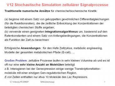
Traditionelle numerische Ansätze für
chemische/biochemische Kinetik (a) beginne mit
einem Satz von gekoppelten gewöhnlichen
Differentialgleichungen (für die Reaktionsraten),
die die zeitliche Entwicklung der Konzentrationen
der beteiligten chemischen Stoffe angeben, (b)
verwende einen geeigneten Integrationsalgorithmus
um, basierend auf den Ratenkonstanten und einem
Satz von Anfangsbedingungen, die Konzentrationen
als Funktion der Zeit zu berechnen Erfolgreiche
Anwendungen für den Hefe Zellzyklus, metabolic
engineering, Modelle der gesamten metabolischen
Pfade (E-cell), ... Großes Problem zelluläre
Prozesse laufen in sehr kleinen Volumina ab und
es ist oft nur eine sehr kleine Anzahl an
Molekülen beteiligt. z.B. Interagieren bei der
Genexpression einige wenige Transkriptionsfaktor-m
oleküle mit einer einzigen Gen-regulatorischen
Region. E.coli Zellen enthalten nur etwa 10
Moleküle des Lac Repressors.
2
berücksichtige stochastische Effekte
(Konsequenz1) ? die Modellierung der Reaktionen
als kontinuierliche Flüsse von Substanzen ist
nicht mehr korrekt. (Konsequenz2) Es können
erhebliche stochastische Fluktuationen
auftreten. Für die Untersuchung der
stochastischen Effekte bei biochemischen
Reaktionen werden stochastische Beschreibungen
der chemischen Kinetik sowie Monte Carlo
Computersimulationen benutzt. Daniel Gillespie
(J Comput Phys 22, 403 (1976) J Chem Phys 81,
2340 (1977)) introduced the exact Dynamic Monte
Carlo (DMC) method that connects the traditional
chemical kinetics and stochastic
approaches. Assuming that the system is well
mixed, the rate constants appearing in these two
methods are related.
3
Dynamic Monte Carlo
In the usual implementation of DMC for kinetic
simulations, each reaction is considered as an
event and each event has an associated
probability of occurring. The probability P(Ei)
that a certain chemical reaction Ei takes place
in a given time interval ?t is proportional to an
effective rate constant k and to the number of
chemical species that can take part in that
event. E.g. the probability of the first-order
reaction X ? Y Z would be k1Nx with Nx
number of species X, and k1 rate constant
of the reaction Similarly, the probability of
the reverse second-order reaction Y Z ?
X would be k2NYNZ.
Resat et al., J.Phys.Chem. B 105, 11026 (2001)
4
Dynamic Monte Carlo
As the method is a probabilistic approach based
on events, reactions included in the DMC
simulations do not have to be solely chemical
reactions. Any process that can be associated
with a probability can be included as an event in
the DMC simulations. E.g. a substrate attaching
to a solid surface can initiate a series of
chemical reactions. One can split the modelling
into the physical events of substrate arrival, of
attaching the substrate, followed by the chemical
reaction steps.
Resat et al., J.Phys.Chem. B 105, 11026 (2001)
5
Basic outline of the direct method of Gillespie
(Step i) generate a list of the
components/species and define the initial
distribution at time t 0. (Step ii) generate a
list of possible events Ei (chemical reactions as
well as physical processes). (Step iii) using
the current component/species distribution,
prepare a probability table P(Ei) of all the
events that can take place. Compute the total
probability P(Ei) probability of event Ei .
(Step iv) Pick two random numbers r1 and r2 ?
0...1 to decide which event E? will occur next
and the amount of time ? by which E? occurs later
since the most recent event.
Resat et al., J.Phys.Chem. B 105, 11026 (2001)
6
Basic outline of the direct method of Gillespie
Using the random number r1 and the probability
table, the event E? is determined by finding the
event that satisfies the relation
The second random number r2 is used to obtain the
amount of time ? between the reactions
As the total probability of the events changes in
time, the time step between occurring steps
varies. Steps (iii) and (iv) are repeated at
each step of the simulation. The necessary
number of runs depends on the inherent noise of
the system and on the desired statistical
accuracy.
Resat et al., J.Phys.Chem. B 105, 11026 (2001)
7
Bacterial Photosynthesis 101
ATPase
Photons
Reaction Center
chemical energy
eHpairs
light energy
outside
inside
Light Harvesting Complexes
cytochrome bc1 complex
ubiquinon cytochrome c2
electronic excitation
H gradient transmembrane potential
electron carriers
8
Modelling as metabolic network
Chemical reactions involved
9
Photosynthesis cycle view
The conversion chain stoichiometries must
match turnovers!
H gradient, transmembrane voltage
electronic excitation
chemical energy
eHpairs
light energy
outside
inside
10
LH1 / LH2 / RC im Lehrbuch
Photonen einfangen
Hu et al, 1998
11
Der Cytochrom bc1 Komplex
die Protonenpumpe"
12
The FoF1-ATP synthase I
at the end of the chain producing ATP from the
H gradient
13
The electron carriers
Cytochrome c electrons from bc1 to RC
heme in a hydrophilic protein shell
3.3 nm diameter
Ubiquinon UQ10 carries electronproton pairs
from RC to bc1
hydrophobic tail
long (2.4 nm) isoprenoid tail
taken from Stryer
14
Tubular membranes photosynthetic vesicleswhere
are the bc1 complexes and the ATPase?
Jungas et al., 1999
15
Chromatophore vesicle typical form in Rh.
sphaeroides
Lipid vesicles 3060 nm diameter H and cyt c
inside
average chromatophore vesicle, 45 nm Ø
surface 6300 nm²
Vesicles are really small!
16
Photon capture rate of LHCs
relative absorption spectrum of LH1/RC and LH2
sun's spectrum at ground (total 1 kW/m²)
multiply
Gerthsen, 1985
Cogdell etal, 2003
Bchl extinction coeff. normalization (?Bchl
2.3 Å2)
Franke, Amesz, 1995
typical growth condition 18 W/m²
Feniouk et al, 2002
LH1 16 3 Bchl ? 14 ?/s LH2 10 3 Bchl ?
10 ?/s
17
LH1 / LH2 / RC native
electron micrograph and density map
Area per per vesicle (45 nm)
LH1 monomer (hexagonal) 146 nm²
LH1 dimer 234 nm²
LH2 monomer 37 nm²
LH12 6 LH2 456 nm² 11
Siebert etal, 2004
125 195 Ų, ? 106
Chromatophore vesicle, 45 nm Ø
surface 6300 nm²
18
Photon processing rate at the RC
Which process limits the RCs turnover?
Unbinding of the quinol ? 25 ms Milano et al.
2003 binding, charge transfer 50 ms per
quinol (estimate) with 2e- H pairs per quinol
? 4050 ?/s per RC ? 22 QH2/s
1 RC can serve 1 LH1 3 LH2 44 ?/s
LH12 6 LH2 ? 456 nm² ? 11 LH1 dimers
including 22 RCs on one vesicle
? 480 Q/s can be loaded _at_ 18 W/m² per vesicle
19
The F1F0-ATP synthase
"mushroom like structures observed in AFM
images"
? ATPase is "visible"
ATPase from ATP/s H/s
chloroblasts lt400 1600
E. coli lt100 400
per turn 1014 H per 3 ATP
20
How much bc1?
measured enzymatic activity per bc1 dimer 84
cyt c are reduced / s
Xiao et al. 2000
in
out
? 1 dimer "pumps" 168 H / s
? 1 dimer can process 42 QH2 / s
400 H / s per ATPase
x5 !!!
? proton generation by 2.4 bc1 dimers per
vesicle enough to drive 1 ATPase
? 11 bc1 dimers per vesicle can be loaded by RCs
safety first! number of bc1 complexes should be
limited by how many protons can be pumped out by
ATPase
21
bc1 Placement Diffusional limits?
Roundtrip times maximal capacity of the carriers
T TRC Tbc1 TDîff
Cytochrome c2
TRC 1 ms
Tbc1 12 ms
TDiff 3 µs
Tround-trip 13 ms ? 3 cyt c per
vesicle sufficient to carry e-s
available 22 cyt c per vesicle
Quinol
TRC 50 ms
Tbc1 23 ms
TDiff 1 ms
Tround-trip 75 ms ? 7 Q per vesicle
sufficient to carry e-s.
? poses no constraints for the position of bc1
available 100 Q per vesicle
22
Proposed setup of a chromatophore vesicle
At the poles green/red the ATPase light blue
the bc1 complexes Increased proton density close
to the ATPase. favors close placing ATPase and
bc1 complexes.
yellow arrows diffusion of the protons out of
the vesicle via the ATPase and to the RCs and
bc1s.
blue small LH2 rings (blue) blue/red Z-shaped
LH1/RC dimers form a linear array around the
equator of the vesicle, determining the
vesicles diameter by their intrinsic curvature.
Geyer, Helms, Biophys. J. (2006) 91, 921
23
reconstituted LH1 dimers in planar lipid membranes
Upper panel drawn after the AFM images of
Scheuring et al (4) of LH1 dimers reconstituted
into planar lipid membranes. The Z-shaped dimers
are seen from their cytoplasmic side. The
average height of the membrane is indicated in
the upper panel by the grey level of the
background. Scheuring et al measured the
distances between the minima of the AFM height
scan to be 38.5 nm and the distance be tween the
lowest and the highest parts to be 3.8 nm.
Lower panel interpretation how alternatingly
oriented LH1 dimers may explain the observed
height scan indicated by the dashed lines. These
values are nicely reproduced by the proposed
arrangement of the LH1 dimers, when one assumes
that they are stiff enough to retain the bending
angle of 26 that they would have on a spherical
vesicle of 45 nm diameter and taking into account
the length of a single LH1 dimer of about 19.5 nm.
24
Photosynthese Lehrbuch-Darstellung
25
Darstellung des photosynthetischen Apparats als
Fließband
Dicke Pfeile Pfad, durch den die
Photonenenergie in chemische Energie umgewandelt
wird, die in ATP gespeichert wird. Abgerundete
Rechtecke kennzeichnen Zwischenzustände. Jede
Umwandlung findet in parallel arbeitenden
Proteinen statt. Ihre Anzahl N mal der
Konversionsrate eines einzelnen Proteins R
bestimmt den gesamten Durchsatz dieses
Schritts. ? eintreffende Photonen, die in den
LHCs aufgefangen werden. E Exzitonen in den
LHCs und in den RCs e-H ElektronenProtonen
Paare, die auf den Quinonen gespeichert
werden. e- sind die Elektronen auf den
Cytochrom c2 pH Protonengradient über die
Membran H Protonen außerhalb des Vesikels
26
Modellierung interner Prozesse am Reaktionszentrum
Die Summe aller Einzelreaktionen mit ihren
individuellen Raten k bestimmt die gesamte
Umsatzrate RRC eines einzelnen RC. Dicke Pfeile
Energiefluss von den Exzitonen durch die
kreisförmigen Änder-ungen der Ladungszustände des
special pair Bchl (P) im RC. Abgerundete
Rechtecke Reservoirs.
27
Parameter
28
Stochastische Dynamiksimulationen II
Produktionsläufe
fester Parametersatz Integriere Ratengleichungen
mit - Gillespie-Algorithmus (Assoziationen) -
Timer-Algorithmus (Reaktionen) 1 Zufallszahl
bestimmt, wann die Reaktion stattfindet.
29
Beispiel Bindung und e- Transfer am
Reaktionszentrum
30
Stochastische Simulationen eines kompletten
Vesikels
Modellvesikel 12 LH1/RC-Monomere 1-6 bc1
Komplexe 1 ATPase 120 Quinone 20 Cytochrom
c2 Integrationszeitschritt 10 ?s Eine Minute
Realzeit zu simulieren benötigt 1,5 Minuten auf
einem Opteron 2.4 GHz Prozessor.
31
Simuliere einen Anstieg der Lichtintensität
Erhöhe Lichtintensität langsam während 1 Minute
von 0 auf 10 W/m2 (Quasi-Gleichgewicht) ? Es
gibt zwei Regimes - eines wird durch das
verfügbare Licht begrenzt - eines durch den
Durchsatz der bc1
Geringe Lichtintensität Linearer Anstieg der
ATP-Produktion mit der Lichtintensität
Hohe Lichtintensität Sättigkeit wird desto
später erreicht umso größer die Anzahl an bc1
Komplexen
Geyer, Lauck, Helms, J. Biotech (im Druck)
32
Oxidationszustand des Cytochrom c2 Pools
geringe Lichtintensität alle 20 Cytochrom
c2 werden durch bc1 reduziert
hohe Lichtintensität RCs sind schneller als die
bc1, die c2s warten auf Elektronen
33
Oxidationszustand des Cytochrom c2 Pools
mehr bc1 Komplexe können mehr Cytochrom c2
beladen.
34
Gesamtzahl an produziertem ATP
Blaue Linie Beleuchtung
Geringe Lichtintensität jede Unterbrechung
stoppt ATP-Produktion Hohe Lichtintensität
Unterbrechungen bis 0.3 s Dauer werden
abgepuffert.
35
c2 Pool wirkt als Puffer
Bei hoher Lichtintensität ist der c2 Pool
vorwiegend oxidiert. Wenn das Licht abgedreht
wird, arbeitet bc1 weiter (c2s beladen, Protonen
pumpen, ATPase zur Produktion von ATP antreiben)
bis der c2 Pool vollkommen reduziert ist.
36
Zusammenfassung
Chromatophoren-Vesikel sind ein ideales
Modellsystem um molekulare Simulationen und
Differentialgleichungsmodelle zu
verknüpfen. Obwohl einige Parameter immer noch
nicht experimentell bekannt sind, kann mit dem
bekannten Wissen ein detailliertes kinetisches
und räumliches Modell erstellt werden. Mit
solchen Systemen kann man testen, wieviel Wissen
über ein System erforderlich ist um es komplett
simulieren zu können. Vorhersagen müssen durch
neue Experimente getestet werden! Solche Tests
sind unbedingt nötig bevor man ein Modell als
korrekt bezeichnen kann.
Recommended
