Ch3. ????(Special Techniques)

1
Ch3. ????(Special Techniques)
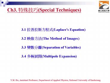
3.1 ???????(Laplaces Equation) 3.2 ????(The
Method of Images) 3.3 ????(Separation of
Variables) 3.4 ????(Multipole Expansion)
2
3.1.1.1 ???????(Laplaces Equation)
Given a stationary charge distribution ,
we can, in principle, calculate the electric
field
where
This integral involves a vector as an integrand
and is, in general, difficult to calculate. In
most cases it is easier to evaluate first the
electrostatic potential V which is defined as
since the integrand of the integral is a
scalar. The corresponding electric field
can then be obtained from the gradient of V since
3
3.1.1.2 ???????(Laplaces Equation)
The electrostatic potential V can only be
evaluated analytically for the simplest charge
configurations. In addition, in many
electrostatic problems, conductors are involved
and the charge distribution is not known
in advance (only the total charge on each
conductor is known).
A better approach to determine the electrostatic
potential is to start with the Poisson's equation

Very often we only want to determine the
potential in a region where ? 0. In this
region Poisson's equation reduces to Laplace's
equation
There are an infinite number of functions that
satisfy Laplace's equation and the appropriate
solution is selected by specifying the
appropriate boundary conditions.
4
3.1.2.1 ??????????(Laplaces Equation in One
Dimension)
In one dimension the electrostatic potential V
depends on only one variable x. The electrostatic
potential V(x) is a solution of the
one-dimensional Laplace equation
The general solution of this equation is V(x)
mx b, where m and b are arbitrary constants.
These constants are fixed when the value of the
potential is specified at two different positions.
Property 1
It is a consequence of the Mean Value Theorem.
5
3.1.2.2 ??????????(Laplaces Equation in One
Dimension)
Property 2
The solution of Laplace's equation can not have
local maxima or minima. Extreme values must occur
at the end points (the boundaries). This is a
direct consequence of property 1.
Property 2 has an important consequence a
charged particle can not be held in stable
equilibrium by electrostatic forces alone
(Earnshaw's Theorem). A particle is in a stable
equilibrium if it is located at a position where
the potential has a minimum value. A small
displacement away from the equilibrium position
will increase the electrostatic potential of the
particle, and a restoring force will try to move
the particle back to its equilibrium position.
However, since there can be no local maxima or
minima in the electrostatic potential, the
particle can not be held in stable equilibrium by
just electrostatic forces.
6
3.1.3 ??????????(Laplaces Equation in Two
Dimension)
In two dimensions the electrostatic potential
depends on two variables x and y. Laplace's
equation now becomes
This equation does not have a simple analytical
solution as the one-dimensional Laplace equation
does. However, the properties of solutions of the
one-dimensional Laplace equation are also valid
for solutions of the two-dimensional Laplace
equation
Property 1
The value of V at a point (x, y) is equal to the
average value of V around this point. If you draw
a circle of any radius R about the point (x,y),
the average value of V on the circle is equal to
the value at the center
Property 2
V has no local maxima or minima all extremes
occur at the boundaries.
7
3.1.4.1 ??????????(Laplaces Equation in Three
Dimension)
In three dimensions the electrostatic potential
depends on three variables x , y , and z.
Laplace's equation now becomes
This equation does not have a simple analytical
solution as the one-dimensional Laplace equation
does. However, the properties of solutions of the
one-dimensional Laplace equation are also valid
for solutions of the three-dimensional Laplace
equation
Property 1
The value of V at a point is equal to the
average value of V over a spherical surface of
radius R at .
Property 2
V has no local maxima or minima all extremes
occur at the boundaries.
8
3.1.4.2 ??????????(Laplaces Equation in Three
Dimension)
Proof of property 1.
The potential at P, generated by charge q, is
equal to
where d is the distance between P and q. Using
the cosine rule we can express d in terms of r, R
and ?.
The potential at P due to charge q is therefore
equal to
The average potential on the surface of the
sphere can be obtained by integrating VP across
the surface of the sphere.
9
3.1.4.3 ??????????(Laplaces Equation in Three
Dimension)
The average potential is equal to
which is equal to the potential due to q at the
center of the sphere. Applying the principle of
superposition it is easy to show that the average
potential generated by a collection of point
charges is equal to the net potential they
produce at the center of the sphere.
10
3.1.4.4 ??????????(Laplaces Equation in Three
Dimension)
Problem 3.3 Find the general solution to
Laplace's equation in spherical coordinates, for
the case where V depends only on r. Then do the
same for cylindrical coordinates.
Laplace's equation in spherical coordinates is
given by
If V is only a function of r, then
Therefore, Laplace's equation can be rewritten as
11
3.1.4.5 ??????????(Laplaces Equation in Three
Dimension)
The solution V of this second-order differential
equation must satisfy the following first-order
differential equation
This differential equation can be rewritten as
The general solution of this first-order
differential equation is
where b is a constant. If V 0 at infinity then
b must be equal to zero, and consequently
12
3.1.4.6 ??????????(Laplaces Equation in Three
Dimension)
Laplace's equation in cylindrical coordinates is
If V is only a function of r, then
Therefore, Laplace's equation can be rewritten as
The solution V of this second-order differential
equation must satisfy the following first-order
differential equation
13
3.1.4.7 ??????????(Laplaces Equation in Three
Dimension)
This differential equation can be rewritten as
The general solution of this first-order
differential equation is
where b is a constant. The constants a and b are
determined by the boundary conditions.
14
3.1.5.1 ?????????(Boundary Conditions and
Uniqueness Theorems)
Consider a volume within which the charge density
is equal to zero. Suppose that the value of the
electrostatic potential is specified at every
point on the surface of this volume. The first
uniqueness theorem states that in this case the
solution of Laplace's equation is uniquely
defined.
Proof
We will consider what happens when there are two
solutions V1 and V2 of Laplace's equation in the
volume. Since V1 and V2 are solutions of
Laplace's equation, we know that
Since both V1 and V2 are solutions, they must
have the same value on the boundary. Thus V1 V2
on the boundary of the volume.
15
3.1.5.2 ?????????(Boundary Conditions and
Uniqueness Theorems)
Now consider a third function V3, which is the
difference between V1 and V2
The function V3 is also a solution of Laplace's
equation. This can be demonstrated easily
The value of the function V3 is equal to zero on
the boundary of the volume since V1 V2 there.
However, property 2 of any solution of Laplace's
equation states that it can have no local maxima
or minima and that the extreme values of the
solution must occur at the boundaries. Since V3
is a solution of Laplace's equation and its value
is zero everywhere on the boundary of the volume,
the maximum and minimum value of V3 must be equal
to zero. Therefore, V3 must be equal to zero
everywhere. This immediately implies that
everywhere
This proves that there can be no two different
functions V1 and V2 that are solutions of
Laplace's equation and satisfy the same boundary
conditions.
16
3.1.5.3 ?????????(Boundary Conditions and
Uniqueness Theorems)
The first uniqueness theorem can only be applied
in those regions that are free of charge and
surrounded by a boundary with a known potential
(not necessarily constant). In many other
electrostatic problems we do not know the
potential at the boundaries of the system.
The second uniqueness theorem states that the
electric field is uniquely determined if the
total charge on each conductor is given and the
charge distribution in the regions between
the conductors is known.
Proof
Suppose that there are two fields and
that are solutions of Poisson's equation in the
region between the conductors. Thus
where ? is the charge density at the point
where the electric field is evaluated.
17
3.1.5.4 ?????????(Boundary Conditions and
Uniqueness Theorems)
The surface integrals of and ,
evaluated using a surface that is just outside
one of the conductors with charge qi, are equal
to qi /?0 .
The difference between and ,
, satisfies the following equations
18
3.1.5.5 ?????????(Boundary Conditions and
Uniqueness Theorems)
Since the potential on the surface of any
conductor is constant, the electrostatic
potential associated with and must
also be constant on the surface of each
conductor. Therefore, V3 V1 -V2 will also be
constant on the surface of each conductor. The
surface integral of V3 over the surface of
conductor i can be written as
Since the surface integral of V3 over the
surface of conductor i is equal to zero, the
surface integral of V3 over all conductor
surfaces will also be equal to zero. The surface
integral of V3 over the outer surface will
also be equal to zero since V3 0 on this
surface. Thus
19
3.1.5.6 ?????????(Boundary Conditions and
Uniqueness Theorems)
Invoking product rule number (5)
Where the volume integration is over all space
between the conductors and the outer surface.
Since is always positive, the volume
integral of can only be equal to zero if
0 everywhere. This implies immediately that
E1 E2 everywhere, and proves the second
uniqueness theorem.
20
3.2.1.1 ???????(The Classic Image Problem)
Consider a point charge q held as a distance d
above an infinite grounded conducting plane.
The electrostatic potential of this system must
satisfy the following two boundary conditions
when
1.
2.
A direct calculation of the electrostatic
potential can not be carried out since the charge
distribution on the grounded conductor is
unknown. Note the charge distribution on the
surface of a grounded conductor does not need to
be zero.
21
3.2.1.2 ???????(The Classic Image Problem)
Consider a second system, consisting of two point
charges with charges q and -q, located at z d
and z -d, respectively. The electrostatic
potential generated by these two charges can be
calculated directly at any point in space.
At a point P (x, y, 0) on the xy plane the
electrostatic potential is equal to
The potential of this system at infinity will
approach zero since the potential generated by
each charge will decrease as 1/r with increasing
distance r. Therefore, the electrostatic
potential generated by the two charges satisfies
the same boundary conditions.
22
3.2.1.3 ???????(The Classic Image Problem)
Since the charge distribution in the region z gt 0
(bounded by the xy plane boundary and the
boundary at infinity) for the two systems is
identical, the corollary of the first uniqueness
theorem states that the electrostatic potential
in this region is uniquely defined. Therefore,
if we find any function that satisfies the
boundary conditions and Poisson's equation, it
will be the right answer. Consider a point (x,
y, z) with z gt 0. The electrostatic potential at
this point can be calculated easily for the
charge distribution shown in last page. It is
equal to
Since this solution satisfies the boundary
conditions, it must be the correct solution in
the region z gt 0. This technique of using image
charges to obtain the electrostatic potential in
some region of space is called the method of
images.
23
3.2.2.1 ???????(Induced Surface Charge)
The electrostatic potential can be used to
calculate the charge distribution on the grounded
conductor. Since the electric field inside the
conductor is equal to zero, the boundary
condition for (see Chapter 2) shows that the
electric field right outside the conductor is
equal to
where ? is the surface charge density and is
the unit vector normal to the surface of the
conductor. Expressing the electric field in
terms of the electrostatic potential V we can
rewrite this equation as
24
3.2.2.2 ???????(Induced Surface Charge)
Substituting the solution for V in this equation
we find
The induced charge distribution is negative and
the charge density is greatest at (x 0, y 0,
z 0). The total charge on the conductor can
be calculated by surface integrating of ?
where r 2 x2 y2. Substituting the expression
for ? in the integral we obtain
25
3.2.3.1 ????(Force and Energy)
As a result of the induced surface charge on the
conductor, the point charge q will be attracted
towards the conductor. Since the electrostatic
potential generated by the charge image charge
system is the same as the charge-conductor system
in the region where z gt 0, the associated
electric field (and consequently the force on
point charge q) will also be the same. The force
exerted on point charge q can be obtained
immediately by calculating the force exerted on
the point charge by the image charge. This force
is equal to
26
3.2.3.2 ????(Force and Energy)
There is however one important difference between
the image-charge system and the real system. This
difference is the total electrostatic energy of
the system. The electric field in the
image-charge system is present everywhere, and
the magnitude of the electric field at (x, y, z)
will be the same as the magnitude of the electric
field at (x, y, -z). On the other hand, in the
real system the electric field will only be non
zero in the region with z gt 0. Since the
electrostatic energy of a system is proportional
to the volume integral of E2, the electrostatic
energy of the real system will be 1/2 of the
electrostatic energy of the image-charge system
(only 1/2 of the total volume has a non-zero
electric field in the real system). The
electrostatic energy of the image-charge system
is equal to
The electrostatic energy of the real system is
therefore equal to
27
3.2.3.3 ????(Force and Energy)
The electrostatic energy of the real system can
also be obtained by calculating the work required
to be done to assemble the system. In order to
move the charge q to its final position we will
have to exert a force opposite to the force
exerted on it by the grounded conductor. The
work done to move the charge from infinity along
the z axis to z d is equal to
which is identical to the result obtained using
the electrostatic potential energy of the image
charge system.
28
3.2.4.1 ???????(Other Image Problem)
Example 3.2

• A point charge q is situated a distance s from
  the center of a grounded conducting sphere of
  radius R.
• Find the potential everywhere.
• b) Find the induced surface charge on the
  sphere, as function of q. Integrate this to get
  the total induced charge.
• c) Calculate the electrostatic energy of this
  configuration.

29
3.2.4.2 ???????(Other Image Problem)
Solution
Image-charge system.
Consider a system consisting of two charges q and
q', located on the z axis at z s and z z',
respectively. The position of point charge q'
must be chosen such that the potential on the
surface of a sphere of radius R, centered at the
origin, is equal to zero (in this case the
boundary conditions for the potential generated
by both systems are identical). The
electrostatic potential at P is equal to
30
3.2.4.3 ???????(Other Image Problem)
The equation above can be rewritten as
The electrostatic potential at Q is equal to
The equation above can be rewritten as
Combining the two expression for q' we obtain
31
3.2.4.4 ???????(Other Image Problem)
The equation above can be rewritten as
The position of the image charge is equal to
The value of the image charge is equal to
32
3.2.4.5 ???????(Other Image Problem)
Now consider an arbitrary point P' on the circle.
The distance between P' and charge q is d and the
distance between P' and charge q' is equal to d'.
Using the cosine rule we can express d and d' in
terms of R, s, and ?
The electrostatic potential at P' is equal to
33
3.2.4.6 ???????(Other Image Problem)
Thus we conclude that the configuration of charge
and image charge produces an electrostatic
potential that is zero at any point on a sphere
with radius R and centered at the origin.
Therefore, this charge configuration produces
an electrostatic potential that satisfies exactly
the same boundary conditions as the potential
produced by the charge-sphere system. Consider
an arbitrary point (r ,?). The distance between
this point and charge q is d and the distance
between this point and charge q' is equal to d'.
These distances can be expressed in terms of r,
s, and ? using the cosine rule
34
3.2.4.7 ???????(Other Image Problem)
The electrostatic potential at (r ,?) will
therefore be equal to
Answer of (a)
(b)
The surface charge density ? on the sphere can be
obtained from the boundary conditions of
where we have used the fact that the electric
field inside the sphere is zero.
35
3.2.4.8 ???????(Other Image Problem)
The equation above can be rewritten as
Substituting the general expression for V into
this equation we obtain
36
3.2.4.9 ???????(Other Image Problem)
The total charge on the sphere can be obtained by
integrating ? over the surface of the sphere.
Answer of (b)
(c)
To obtain the electrostatic energy of the system
we can determine the work it takes to assemble
the system by calculating the path integral of
the force that we need to exert in charge q in
order to move it from infinity to its final
position (z s).
37
3.2.4.10 ???????(Other Image Problem)
Charge q will feel an attractive force exerted by
the induced charge on the sphere. The strength of
this force is equal to the force on charge q
exerted by the image charge q'.
This force is equal to
The force that we must exert on q to move it from
infinity to its current position is opposite to
. The total work required to move the charge
is therefore equal to
Answer of (c)
38
3.3.1.1 ?????????(Separation of Variables
Cartesian Coordinates)
Example 3.3
Two infinite, grounded, metal plates lie parallel
to the xz plane, one at y 0, the other at y a
(see Figure below). The left end, at x 0, is
closed off with an infinite strip insulated from
the two plates and maintained at a specified
potential V0(y). Find the potential inside this
"slot".
a
V0(y)
39
3.3.1.2 ?????????(Separation of Variables
Cartesian Coordinates)
The electrostatic potential in the slot must
satisfy the three-dimensional Laplace equation.
However, since V does not have a z dependence,
the three-dimensional Laplace equation reduces to
the two-dimensional Laplace equation
The boundary conditions for the solution of
Laplace's equation are 1. V(x, y 0) 0
(grounded bottom plate). 2. V(x, y a) 0
(grounded top plate). 3. V(x 0, y) V0(y)
(plate at x 0). 4. When
.
These four boundary conditions specify the value
of the potential on all boundaries surrounding
the slot and are therefore sufficient to uniquely
determine the solution of Laplace's equation
inside the slot.
40
3.3.1.3 ?????????(Separation of Variables
Cartesian Coordinates)
Consider solutions of the following form
If this is a solution of the two-dimensional
Laplace equation then we must require that
This equation can be rewritten as
The first term of the left-hand side of this
equation depends only on x while the second term
depends only on y.
41
3.3.1.4 ?????????(Separation of Variables
Cartesian Coordinates)
If the above equation must hold for all x and y
in the slot we must require that
The differential equation for X can be rewritten
as
If C1 is a negative number then this equation can
be rewritten as
where
The most general solution of this equation is
However, this function is an oscillatory function
and does not satisfy boundary condition 4,
which requires that V approaches zero when x
approaches infinity.
42
3.3.1.5 ?????????(Separation of Variables
Cartesian Coordinates)
We therefore conclude that C1 can not be a
negative number. If C1 is a positive number then
the differential equation for X can be written as
where
The most general solution of this equation is
This solution will approach zero when x
approaches infinity if A 0. Thus
The solution for Y can be obtained by solving the
following differential equation
43
3.3.1.6 ?????????(Separation of Variables
Cartesian Coordinates)
The most general solution of the above equation is
Therefore, the general solution for the
electrostatic potential V(x,y) is equal
where we have absorbed the constant B into the
constants C and D. The constants C and D must be
chosen such that the remaining three boundary
conditions (1, 2, and 3) are satisfied.
The first boundary condition requires that V(x, y
0) 0
which requires that C 0.
44
3.3.1.7 ?????????(Separation of Variables
Cartesian Coordinates)
The second boundary condition requires that V(x,
y a) 0
which requires that sin ka 0. This condition
limits the possible values of k
where n 1, 2, 3,
Note negative values of k are not allowed since
exp(-kx) approaches zero at infinity only if k gt0.
However, since n can take on an infinite number
of values, there will be an infinite number of
solutions of Laplace's equation satisfying
boundary conditions 1, 2 and 4. The most
general form of the solution of Laplace's
equation will be a linear superposition of all
possible solutions. Thus
45
3.3.1.8 ?????????(Separation of Variables
Cartesian Coordinates)
To satisfy boundary condition 3 we must require
that
Multiplying both sides by sin(n?y/a) and
integrating each side between y 0 and y a we
obtain
The integral on the left-hand side of this
equation is equal to zero for all values of n
except n n. Thus
where
46
3.3.1.9 ?????????(Separation of Variables
Cartesian Coordinates)
The coefficients Dn can thus be calculated
easily
The coefficients Dn are called the Fourier
coefficients of V0(y)
The solution of Laplace's equation in the slot is
therefore equal to
where
47
3.3.1.10 ?????????(Separation of Variables
Cartesian Coordinates)
Problem 3.12
Find the potential in the infinite slot of
Example 3.3 if the boundary at x 0 consists to
two metal stripes one, from y 0 to y a/2, is
held at constant potential V0 , and the other,
from y a/2 to y a is at potential -V0 .
The boundary condition at x 0 is
The Fourier coefficients of the function V0(y)
are equal to
48
3.3.1.11 ?????????(Separation of Variables
Cartesian Coordinates)
The values for the first four G coefficients are
It is easy to see that Gn 4 Gn and therefore
we conclude that
The Fourier coefficients Dn are thus equal to
The electrostatic potential is thus equal to
49
3.3.2.1 ?????????(Separation of Variables
Spherical Coordinates)
Consider a spherical symmetric system. If we want
to solve Laplace's equation it is natural to use
spherical coordinates. Assuming that the system
has azimuthal symmetry ( ?V / ?? 0) Laplace's
equation reads
Consider the possibility that the general
solution of this equation is the product of a
function R(r), which depends only on the distance
r, and a function ?(? ), which depends only on
the angle ?
Substituting this "solution" into Laplace's
equation we obtain
50
3.3.2.2 ?????????(Separation of Variables
Spherical Coordinates)
The first term in this expression depends only on
the distance r while the second term depends only
on the angle ?. This equation can only be true
for all r and ? if
Consider a solution for R of the following form
where A and k are arbitrary constants.
Substituting this expression in the differential
equation for R(r) we obtain
51
3.3.2.3 ?????????(Separation of Variables
Spherical Coordinates)
This equation gives us the following expression
for k
The general solution for R(r) is thus given by
where A and B are arbitrary constants.
52
3.3.2.4 ?????????(Separation of Variables
Spherical Coordinates)
The angle dependent part of the solution of
Laplace's equation must satisfy the following
equation
The solutions of this equation are known as the
Legendre polynomial P (cos?).
P (cos?) is most conveniently defined by the
Rodrigues formula
53
3.3.2.5 ?????????(Separation of Variables
Spherical Coordinates)

• The Legendre polynomials have the following
  properties
• If even,
• If odd,
• for all
• 4.
  or
  .

54
3.3.2.6 ?????????(Separation of Variables
Spherical Coordinates)
Combining the solutions for R(r) and ?(? ) we
obtain the most general solution of Laplace's
equation in a spherical symmetric system with
azimuthal symmetry
Problem 3.18
The potential at the surface of a sphere is given
by
where k is some constant. Find the potential
inside and outside the sphere, as well as the
surface charge density ?(?) on the sphere.
(Assume that there is no charge inside or outside
of the sphere.)
55
3.3.2.7 ?????????(Separation of Variables
Spherical Coordinates)
The most general solution of Laplace's equation
in spherical coordinates is
First consider the region inside the sphere (r lt
R). In this region since otherwise
V(r,?) would blow up at r 0. Thus
The potential at r R is therefore equal to
Using trigonometric relations we can rewrite
56
3.3.2.8 ?????????(Separation of Variables
Spherical Coordinates)
Substituting the above expression in the equation
for V(R,?) we obtain
This equation immediately shows that A 0
unless 1 or 3.
If 1 or 3,
The electrostatic potential inside the sphere is
therefore equal to
57
3.3.2.9 ?????????(Separation of Variables
Spherical Coordinates)
Now consider the region outside the sphere (r gt
R). In this region since otherwise
V(r,?) would blow up at infinity. The solution of
Laplace's equation in this region is therefore
equal to
The potential at r R is therefore equal to
This equation immediately shows that B 0
unless 1 or 3.
If 1 or 3,
The electrostatic potential outside the sphere is
thus equal to
58
3.3.2.10 ?????????(Separation of Variables
Spherical Coordinates)
The charge density on the sphere can be obtained
using the boundary conditions for the electric
field at a boundary
Since this boundary
condition can be rewritten as
The first term on the left-hand side of this
equation can be calculated using the
electrostatic potential just obtained
59
3.3.2.11 ?????????(Separation of Variables
Spherical Coordinates)
In the same manner we obtain
Therefore,
The charge density on the sphere is thus equal to
60
3.3.2.12 ?????????(Separation of Variables
Spherical Coordinates)
Example Problem 3.19
Suppose the potential V0(?) at the surface of a
sphere is specified, and there is no charge
inside or outside the sphere. Show that the
charge density on the sphere is given by where
Solution
First consider the electrostatic potential inside
the sphere. The electrostatic potential in this
region is given by
61
3.3.2.13 ?????????(Separation of Variables
Spherical Coordinates)
and the boundary condition is
The coefficients can be determined by
multiplying both sides of this equation by
Pn(cos?)sin? and integrating with respect to ?
between ? 0 and ? ?
Remember that
Thus
62
3.3.2.14 ?????????(Separation of Variables
Spherical Coordinates)
In the region outside the sphere the
electrostatic potential is given by
and the boundary condition is
The coefficients can be determined by
multiplying both sides of this equation by
Pn(cos?)sin? and integrating with respect to ?
between ? 0 and ? ?
Thus
63
3.3.2.15 ?????????(Separation of Variables
Spherical Coordinates)
The charge density ?(?) on the surface of the
sphere is equal to
Differentiating V(r,?) with respect to r in the
region r gt R we obtain
Differentiating V(r,?) with respect to r in the
region r lt R we obtain
64
3.3.2.16 ?????????(Separation of Variables
Spherical Coordinates)
where
65
3.3.3.1 ?????????(Separation of Variables
Cylindrical Coordinates)
Example Problem 3.23
Solve Laplace's equation by separation of
variables in cylindrical coordinates, assuming
there is no dependence on z (cylindrical
symmetry). Make sure that you find all solutions
to the radial equation.
For a system with cylindrical symmetry the
electrostatic potential does not depend on z.
This immediately implies that ?V / ?z 0. Under
this assumption Laplace's equation reads
Consider as a possible solution of V
66
3.3.3.2 ?????????(Separation of Variables
Cylindrical Coordinates)
Substituting this solution into Laplace's
equation we obtain
Multiplying each term in this equation by r2 and
dividing by R(r)?(?) we obtain
The first term in this equation depends only on r
while the second term in this equation depends
only on ?. This equation can therefore be only
valid for every r and every ? if each term is
equal to a constant. Thus we require that
67
3.3.3.3 ?????????(Separation of Variables
Cylindrical Coordinates)
First consider the case in which ? -m2 lt 0. The
differential equation for ?(?) can be rewritten as
The most general solution of this differential
solution is
However, in cylindrical coordinates we require
that any solution for a given ? is equal to the
solution for ?2?. Obviously this condition is
not satisfied for this solution, and we conclude
that ? m2 0.
The differential equation for ?(?) can be
rewritten as
68
3.3.3.4 ?????????(Separation of Variables
Cylindrical Coordinates)
The most general solution of this differential
solution is
The condition that ?m(?) ?m(?2?) requires that
m is an integer.
Now consider the radial function R(r). We will
first consider the case in which ? m2 gt 0.
Consider the following solution for R(r)
Substituting this solution into the previous
differential equation we obtain
Therefore, the constant k can take on the
following two values
69
3.3.3.5 ?????????(Separation of Variables
Cylindrical Coordinates)
The most general solution for R(r) under the
assumption that m2 gt 0 is therefore
Now consider the solutions for R(r) when m2 0.
In this case we require that
If a0 0 then the solution of this differential
equation is
If a0 ? 0 then the solution of this differential
equation is
70
3.3.3.6 ?????????(Separation of Variables
Cylindrical Coordinates)
Combining the solutions obtained for m2 0 with
the solutions obtained for m2 gt 0 we conclude
that the most general solution for R(r) is given
by
Therefore, the most general solution of Laplace's
equation for a system with cylindrical symmetry is
71
3.3.3.7 ?????????(Separation of Variables
Cylindrical Coordinates)
Example Problem 3.25
A charge density ?(?) a sin(5?) (where a is a
constant) is glued over the surface of an
infinite cylinder of radius R. Find the potential
inside and outside the cylinder.
In the region inside the cylinder the coefficient
Bm must be equal to zero since otherwise V(r,?)
would blow up at r 0. For the same reason a0
0. Thus
In the region outside the cylinder the
coefficients Am must be equal to zero since
otherwise V(r, ?) would blow up at infinity. For
the same reason a0 0. Thus
Since V(r,?) must approach 0 when r approaches
infinity, we must also require that bout, 0 is
equal to 0.
72
3.3.3.8 ?????????(Separation of Variables
Cylindrical Coordinates)
The charge density on the surface of the cylinder
is equal to
Differentiating V(r,?) in the region r gt R and
setting r R we obtain
Differentiating V(r,?) in the region r lt R and
setting r R we obtain
The charge density on the surface of the cylinder
is therefore equal to
73
3.3.3.9 ?????????(Separation of Variables
Cylindrical Coordinates)
Since the charge density is proportional to
sin(5?) we can conclude immediately that Cin,m
Cout ,m 0 for all m and that Din,m Dout ,m
0 for all m except m 5.
Therefore
This requires that
A second relation between Din, 5 and Dout, 5 can
be obtained using the condition that the
electrostatic potential is continuous at any
boundary. This requires that
74
3.3.3.10 ?????????(Separation of Variables
Cylindrical Coordinates)
Thus
We now have two equations with two unknown, Din,
5 and Dout, 5 , which can be solved with the
following result
The electrostatic potential inside the cylinder
is thus equal to
The electrostatic potential outside the cylinder
is thus equal to
75
3.4.1.1 ????(Multipole Expansion)
Consider a given charge distribution ?. The
potential at a point P (see Figure below) is
equal to
where d is the distance between P and a
infinitesimal segment of the charge distribution.
d can be written as a function of r, r' and ?
so
76
3.4.1.2 ????(Multipole Expansion)
At large distances from the charge distribution r
gtgt r and consequently r/r ltlt1. Using the
following expansion for
we can rewrite 1/d as
77
3.4.1.3 ????(Multipole Expansion)
Using the expansion of 1/d we can rewrite the
electrostatic potential at P as
This expression is valid for all r (not only r gtgt
r). However, if r gtgt r' then the potential at P
will be dominated by the first non-zero term in
this expansion. This expansion is known as the
multipole expansion.
In the limit of r gtgt r only the first terms in
the expansion need to be considered
The first term in this expression, proportional
to 1/r, is called the monopole term. The second
term in this expression, proportional to 1/r2, is
called the dipole term. The third term in this
expression, proportional to 1/r3, is called the
quadrupole term.
78
3.4.2.1 ???(The Monopole Term)
If the total charge of the system is non zero,
then the electrostatic potential at large
distances is dominated by the monopole term
where Q is the total charge of the charge
distribution.
The electric field associated with the monopole
term can be obtained by calculating the gradient
of V(P)
79
3.4.2.2 ???(The Dipole Term)
If the total charge of the charge distribution is
equal to zero (Q 0), then the monopole term in
the multipole expansion will be equal to zero. In
this case the dipole term will dominate the
electrostatic potential at large distances.
Since ? is the angle between r and r ' we can
rewrite rcos? as
The electrostatic potential at P can therefore be
rewritten as
In this expression p is the dipole moment of the
charge distribution which is defined as
80
3.4.2.3 ???(The Dipole Term)
The electric field associated with the dipole
term can be obtained by calculating the gradient
of V(P)
81
3.4.2.4 ???(The Dipole Term)
Consider a system of two point charges shown in
Figure below. The total charge of this system is
zero, and therefore the monopole term is equal to
zero. The dipole moment of this system is equal to
The dipole moment of a charge distribution
depends on the origin of the coordinate system
chosen. Consider a coordinate system S and a
charge distribution ?. The dipole moment of this
charge distribution is equal to
82
3.4.2.5 ???(The Dipole Term)
A second coordinate system S' is displaced by
with respect to S
The dipole moment of the charge distribution in
S' is equal to
This equation shows that if the total charge of
the system is zero (Q 0) then the dipole moment
of the charge distribution is independent of the
choice of the origin of the coordinate system.
83
3.4.2.6 ???(The Dipole Term)
Example Problem 3.40
A thin insulating rod, running from z -a to z
a, carries the following line charges
In each case, find the leading term in the
multipole expansion of the potential.
84
3.4.2.7 ???(The Dipole Term)
a) The total charge on the rod is equal to
Since Qtot ? 0, the monopole term will dominate
the electrostatic potential at large distances.
Thus
b) The total charge on the rod is equal to zero.
Therefore, the electrostatic potential at large
distances will be dominated by the dipole term
(if non-zero). The dipole moment of the rod is
equal to
Since the dipole moment of the rod is not equal
to zero, the dipole term will dominate the
electrostatic potential at large distances.
Therefore
85
3.4.2.8 ???(The Dipole Term)
c) For this charge distribution the total charge
is equal to zero and the dipole moment is equal
to zero. The electrostatic potential of this
charge distribution is dominated by the
quadrupole term.
-
The electrostatic potential at large distance
from the rod will be equal to
86
3.4.2.9 ???(The Dipole Term)
Example Problem 3.27
Four particles (one of charge q, one of charge
3q, and two of charge -2q) are placed as shown in
Figure below, each a distance d from the origin.
Find a simple approximate formula for the
electrostatic potential, valid at a point P far
from the origin.
d
The total charge of the system is equal to zero
and therefore the monopole term in the multipole
expansion is equal to zero. The dipole moment of
this charge distribution is equal to
87
3.4.2.10 ???(The Dipole Term)
The Cartesian coordinates of P are
The scalar product between and is
therefore
The electrostatic potential at P is therefore
equal to