
Previous approach to supervised learning (Parametric approach) : PowerPoint PPT Presentation
1 / 64
Title: Previous approach to supervised learning (Parametric approach) :
1
LINEAR DISCRIMINANT FUNCTIONS
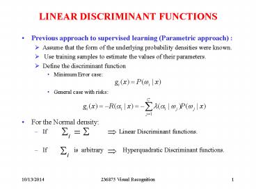
- Previous approach to supervised learning
(Parametric approach) - Assume that the form of the underlying
probability densities were known. - Use training samples to estimate the values of
their parameters. - Define the discriminant function
- Minimum Error case
- General case with risks
- For the Normal density
- If
Linear Discriminant functions. - If is arbitrary
Hyperquadratic Discriminant functions.
2
LINEAR DISCRIMINANT FUNCTIONS cont.
- In this lecture we assume that we know the proper
form of the discriminant functions, and use the
samples to estimate the parameters. This approach
does not require knowledge of the forms of
underlying pdf's. - We will consider only linear discriminant
functions. Linear discriminant functions are
relatively easy to compute.
3
LINEAR DISCRIMINANT FUNCTIONS AND DECISION
SURFACES The 2-Category Case
- A linear discriminant function can be written as
- where w weight vector, w0 bias or
threshold - ( in the next lectures we shall call it b to
be close to SVM terminology) - A 2-class linear classifier implements the
following decision rule - Decide w1 if g(x)gt0 and w2
if g(x)lt0.
4
The 2-Category Case cont.
- A simple
linear classifier - The equation g(x) 0 defines the decision
surface that separates points - assigned to w1 from points assigned to w2.
- When g(x) is linear, this decision surface is a
Hyperplane (H).
5
The 2-Category Case cont.
- H divides the feature space into 2 half spaces
R1 for w1, and R2 for w2. - If x1 and x2 are both on the decision surface
- w is normal to any vector lying in the
hyperplane
6
The 2-Category Case cont.
7
The 2-Category Case cont.
- If we express x as
- where xp is the normal projection of x onto H,
and r is the algebraic - distance from x to the hyperplane. Since
g(xp)0, we have - or
- r is signed distance r gt 0 if x falls in R1
, r lt 0 if x falls in R2 . - Distance from the origin to the hyperplane is
w0/w .
8
The Multicategory Case
- 2 approaches to extend the linear discriminant
functions approach to the multicategory case - Reduce the problem to C-1 two-class problems
Problem i Find the functions that separates
points assigned to w i - from those not assigned to w i.
- 2. Find the c(c-1)/2 linear discriminants,
one for every pair of classes - Both approaches can lead to regions in which the
classification is undefined ( see the Figure ).
9
The Multicategory Case
- dichotomy
- dichotomy
10
The 2-Category Case cont.
- Define c linear discriminant functions
- Classifier
- in case of equal scores, the classification
is left undefined. - The resulting classifier is called a Linear
Machine. - A linear machine divides the feature space into c
decision regions, with gi(x) being the largest
discriminant if x is in region Ri. - If Ri and Rj are contiguous, the boundary between
them is a portion of the hyperplane Hij defined
by
11
The 2-Category Case cont.
- It follows that is normal
to Hij - The signed distance from x to Hij is given by
- There are c(c-1)/2 pairs of regions. They are
convex . - Not all regions in real life are contiguous, and
the total number of hyperplane segments appearing
in the decision surfaces is often fewer than
c(c-1)/2. -
Decision boundaries - 3-class
problem 5-class problem
12
GENERALIZED LINEAR DISCRIMINANT FUNCTIONS
- The linear discriminant function g(x) can be
written as - By adding d(d1)/2 additional terms involving the
products of pairs of components of x, we obtain
the quadratic discriminant function - The separating surface defined by g(x)0 is a
second-degree or hyperquadric surface. - By continuing to add terms such as
we can obtain the class of polynomial
discriminant functions.
13
GENERALIZED LINEAR DISCRIMINANT FUNCTIONS
- Polynomial functions can be thought of as
truncated series expansions of some arbitrary
g(x). - The generalized linear discriminant function is
defined as - where is a -dimensional weight
vector, and is an arbitrary function
of x. - The resulting discriminant function is not linear
in x, but it is linear in y. - The functions map points in d
-dimensional x-space to points in -dimensional
y-space.
14
Example1
- Let the quadratic discriminant function be
- The 3-dimensional vector y is then given by
15
Example2.
- Whenever is degenerate
(everywhere 0, but on the curve is infinite) . - The plane H defined by divides
the y-space into 2 decision regions R1 and R2. - If
- Decision regions in the original x-space are
nonconvex - In y-space they are convex.
16
THE TWO-CATEGORY LINEARLY-SEPARABLE CASE
- where x01.
- Let -
augmented feature vector (trivial mapping from
d-dimensional x-space to (d1)-dimensional
y-space) and
augmented weight vector. Then
. The hyperplane decision surface
defined passes through the
origin in y-space. The distance from any point y
to is given by , or - Because this
distance is less then distance from x to H. The
problem of finding w0,w is changed to a problem
of - finding vector
17
THE TWO-CATEGORY LINEARLY-SEPARABLE CASE
- Suppose that we have a set of n samples
some labeled w1 and some labeled w2. - Use these training samples to determine the
weights . - Look for a weight vector that classifies all the
samples correctly. - If such a weight vector exists, the samples are
said to be linearly separable. A sample
yi is classified correctly if - or
18
THE TWO-CATEGORY LINEARLY-SEPARABLE CASE
- If we replace all the samples labeled w2 by their
negatives, then we can look for a weight vector
such that for all the
samples. Such a weight vector is called a
separating vector or more generally a solution
vector. - Each sample places a constraint on the possible
location of a solution vector. - defines a hyperplane through the
origin having as a normal vector. - The solution vector (if it exists) must be on the
positive side of every hyperplane - Intersection of the n half-spaces Solution
Region
19
THE TWO-CATEGORY LINEARLY-SEPARABLE CASE
- Any vector that lies in the solution region is a
solution vector. - The solution vector (if it exists) is not unique.
- We can impose additional requirements to find a
solution vector closer to the middle of the
region (the resulting solution is more likely to
classify new test samples correctly).
20
THE TWO-CATEGORY LINEARLY-SEPARABLE CASE
- Seek a unit-length weight vector that maximizes
the minimum distance from the samples to the
separating plane. - Seek the minimum-length weight vector satisfying
- The solution region shrinks by margins b/yi
- The new
solution lies within the previous region
21
GRADIENT DESCENT PROCEDURES
- Define a criterion function that is
minimized if is a solution vector (
for all samples). - Start with some arbitrarily chosen weight vector
. - Compute the gradient vector .
- The next value is obtained by moving
a distance from - in the direction of steepest descent
(i.e. along the negative of the gradient) . - In general, is obtained from
using - where is learning rate.
22
GRADIENT DESCENT algorithm
- begin initialize
- do
- until
- return
- end
- How to set the learning rate ? Suppose
23
GRADIENT DESCENT algorithm
- where is the Hessian
matrix evaluated at - Substituting into (2) from
(1) - By equating to zero a derivative with respect to
we - get
24
Newtons algorithm.
- Choose a(k1) to minimize (2) equate to
- zero a derivative of the r.h.s. of (2) with
respect to a - and then substitute a(k1) in place of a
25
Newtons algorithm.
- begin initialize
- do
- until
- return
- end
- Newtons algorithm gives a greater improvement
per step, then gradient descent, but is not
applicable , when Hessian - is singular and also takes O(d3) time.
26
MINIMIZING THE PERCEPTRON CRITERION FUNCTION
- Perceptron criterion function
- is the set of samples misclassified
by . - If no samples are misclassified, is
empty, and - Since if is
misclassified, is never negative,
and is zero only if is a solution vector.
- Geometrically, is proportional to
the sum of the distances from the misclassified
samples to the decision boundary. - Since the update
rule becomes - where is the set of samples
misclassified by .
27
The Batch Perceptron Algorithm
- begin initialize
- do
- until
- return
- end
28
Perceptron Algorithm cont.
- Sequence of
misclassified samples y2,y3,y1,y3
29
The Fixed-Increment Single-Sample Perceptron
- begin initialize
- do
- until all patterns properly
classified - return a
- end
30
Perceptron Algorithm - Comments
- The perceptron algorithm adjusts the parameters
only when it encounters an error, i.e.
misclassified training example . - Correctly classified examples can be ignored.
- The learning rate can be chosen arbitrary,
it will only impact on the norm of the final
vector w (and the corresponding magnitude of w0). - The final weight vector is a linear combination
of training points
31
RELAXATION PROCEDURES
- Another criterion function that is minimized when
is a solution vector - where still denotes the set of
training samples misclassified by . - The advantages of Jq over Jp is that its gradient
is continuous, whereas the gradient of Jp is not.
Jq presents a smoother surface to search. - Disadvantages
- Jq is so smooth near the boundary of the solution
region that the sequence of weight vectors can
converge to a point on the boundary a0 - The value of Jq can be dominated by the longest
sample vectors.
32
RELAXATION PROCEDURES cont.
- Solution of these problems
- Use the following criterion function
- where denotes the set of
samples for which - If is empty, define .
- Jr is never negative .
- Jr 0 if and only if for
all the training samples. - The gradient of Jr is given by
33
RELAXATION PROCEDURES cont.
- Update rule for batch relaxation with margin
34
Nonseparable Behavior
- The Perceptron and Relaxation procedures are
methods for finding a separating vector when the
samples are linearly separable. They are error
correcting procedures. - Even if a separating vector is found for the
training samples, it does not follow that the
resulting classifier will perform well on
independent test data. - To ensure that the performance on training and
test data will be similar, many training samples
should be used. - Unfortunately, sufficiently large training
samples are almost certainly not linearly
separable. - No weight vector can correctly classify every
sample in a nonseparable set
35
Nonseparable Behavior
- The corrections in the Perceptron and Relaxation
procedures can never cease if set is
nonseparable. - If we choose
- then we can get acceptable performance on
nonseparable problems while preserving the
ability to find a separating vector on separable
problems. - The rate at which approaches zero is
important - Too slow Results will be sensitive to those
training samples that render the set
nonseparable. - Too fast Weight vector may converge prematurely
with less than optimal results. - We can make a function of recent
performance, decreasing it as performance
improves. - We can choose
36
MINIMUM SQUARED ERROR PROCEDURES
- The MSE approach sacrifices the ability to obtain
a separating vector for good compromise
performance on both separable and nonseparable
problems. - The Perceptron and Relaxation procedures use the
misclassified samples only. - Previously, we sought a weight vector
making all of the inner products - In the MSE procedure, we will try to make
, where bi are some arbitrarily
specified positive constants. - Using matrix notation
37
MINIMUM SQUARED ERROR PROCEDURES cont.
- Using matrix notation
- or
- If Y is nonsingular, then
- Unfortunately, Y is not a square matrix, usually
with more rows than columns.
38
MINIMUM SQUARED ERROR PROCEDURES cont.
- When there are more equations than unknowns,
is overdetermined, and ordinarily no exact
solution exists. - We can seek a weight vector that minimizes
some function of an error vector e - Minimize the squared length of the error vector,
which is equivalent to minimizing the
sum-of-squared-error criterion function - Setting the gradient equal to zero, we get the
following necessary condition
39
MINIMUM SQUARED ERROR PROCEDURES cont.
- is a square matrix, and often
nonsingular. Therefore, we can solve for
using
40
MINIMUM SQUARED ERROR PROCEDURES cont.
- where
- is called pseudoinverse of Y.
- is defined more generally by
- It can be shown that this limit always exists
is - MSE solution to
- Different choices of b give the solution
different properties.
41
Example
- Suppose we have the following
two-dimensional points for the two categories
w1 and , and w2
and -
Four training points -
and decision boundary
4
R2
3
2
1
R1
1
2
3
4v
0
42
Example
- Our matrix Y is
- Pseudoinverse is
- If arbitrarily let all the margins be equal
- we shall find the solution
43
Relation to Fishers Linear Discriminant
- With special choice of the vector b, the MSE is
connected to Fishers linear discriminant. - Assume n d-dimensional samples
n1 are from D1 and n2 are from D2 - The matrix Y can be written
- where 1i is a column vector of ni ones, and
Xi is an ni-by-d matrix which rows are labeled
wi. We partition a and b
44
Relation to Fishers Linear Discriminant cont.
- Lets write
- Remember that sample mean is
- and
45
Relation to Fishers Linear Discriminant cont.
- We can multiply matrices in (4)
- From the first row we have
- and from the second
46
Relation to Fishers Linear Discriminant cont.
- But the vector
is in the direction of - for any value of
, thus we can write - for some scalar a .
- Then (10) yields
- which is proportional to the Fisher linear
discriminant. The decision rule is decide
otherwise decide
47
THE WIDROW-HOFF PROCEDURE
- The criterion function
could be minimized by a gradient
descent procedure. - Advantages
- Avoids the problems that arise when is
singular. - Avoids the need for working with large matrices.
- Since
- a simple update rule would be
- If we consider the samples sequentially
48
THE WIDROW-HOFF PROCEDURE
- Widrow-Hoff or LMS (Least-Mean-Square) procedure
- Initialize
- do
- until
- return
- end
49
Content
Linear Learning Machines and SVM The Perceptron
Algorithm revisited Functional and Geometric
Margin Novikoff theorem Dual Representation Learni
ng in the Feature Space Kernel-Induced Feature
Space Making Kernels The Generalization Problem
Probably Approximately Correct
Learning Structural Risk Minimization
50
Linear Learning Machines and SVM
- Basic Notations
- Input space
- Output space for
classification - for regression
- Hypothesis
- Training Set
- Test error also R(a)
- Dot product
51
Basic Notations cont.
- Learning machine any function estimation
algorithm, - training parameter estimation procedure,
- testing computation of function value,
- performance generalization accuracy (i.e.
error rate as - test set size tends to infinity
52
The Perceptron Algorithm
revisited
- Linear separation
- of the input space
- The algorithm requires that the input patterns
are linearly separable, - which means that there exist linear discriminant
function which has - zero training error. We assume that this is the
case.
53
The Perceptron Algorithm (primal
form)
- initialize
- repeat
- error false
- for i1..l
- if
then - error true
- end if
- end for
- until (errorfalse)
- return k,(wk,bk) where k is the number of
mistakes
54
The Perceptron Algorithm
Comments
- The perceptron works by adding misclassified
positive or subtracting misclassified negative
examples to an arbitrary weight vector, which
(without loss of generality) we assumed to be the
zero vector. So the final weight vector is a
linear combination of training points - where, since the sign of the coefficient of
is given by label yi, the are
positive values, proportional to the number of
times, misclassification of has caused the
weight to be updated. It is called the embedding
strength of the pattern .
55
Functional and Geometric
Margin
- The notion of margin of a data point w.r.t. a
linear discriminant will turn out to be an
important concept. - The functional margin of a linear discriminant
(w,b) w.r.t. a labeled pattern
is defined as - If the functional margin is negative, then the
pattern is incorrectly classified, if it is
positive then the classifier predicts the correct
label. - The larger the further away xi is from
the discriminant. - This is made more precise in the notion of the
geometric margin
56
Functional and Geometric
Margin cont.
The geometric margin of The
margin of a training set two
points
57
Functional and Geometric
Margin cont.
- which measures the Euclidean distance of a
point from the decision boundary. - Finally, is called the
(functional) margin of (w,b) - w.r.t. the data set S(xi,yi).
- The margin of a training set S is the maximum
geometric margin over all hyperplanes. A
hyperplane realizing this maximum is a maximal
margin hyperplane. - Maximal Margin
Hyperplane
58
Novikoff theorem
- Theorem
- Suppose that there exists a vector
and a bias term such that
the margin on a (non-trivial) data set S is at
least , i.e. - then the number of update steps in the
perceptron algorithm is at most - where
59
Novikoff theorem
cont.
- Comments
- Novikoff theorem says that no matter how small
the margin, if a data set is linearly separable,
then the perceptron will find a solution that
separates the two classes in a finite number of
steps. - More precisely, the number of update steps (and
the runtime) will depend on the margin and is
inverse proportional to the squared margin. - The bound is invariant under rescaling of the
patterns. - The learning rate does not matter.
60
Dual
Representation
- The decision function can be rewritten as
follows - And also the update rule can be rewritten as
follows - The learning rate only influence the overall
scaling of the hyperplanes, it does no effect
algorithm with zero starting vector, so we can
put
61
Duality First Property of
SVMs
- DUALITY is the first feature of Support Vector
Machines - SVM are Linear Learning Machines represented in a
dual fashion - Data appear only inside dot products (in decision
- function and in training algorithm)
- The matrix is
called Gram matrix
62
Limitations of Linear
Classifiers
- Linear Learning Machines (LLM) cannot deal with
- Non-linearly separable data
- Noisy data
- This formulation only deals with vectorial data
63
Limitations of Linear
Classifiers
- Neural networks solution multiple layers of
thresholded linear functions multi-layer neural
networks. Learning algorithms back-propagation. - SVM solution kernel representation.
- Approximation-theoretic issues are independent
of the learning-theoretic ones. Learning
algorithms are decoupled from the specifics of
the application area, which is encoded into
design of kernel.
64
Learning in the Feature
Space
- Map data into a feature space where they are
linearly separable (i.e.
attributes features)
Recommended
