Deterministic ModelsStochastic Models

1
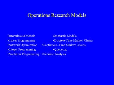
Operations Research Models
Deterministic Models Stochastic Models Linear
Programming Discrete-Time Markov
Chains Network Optimization Continuous-Time
Markov Chains Integer Programming Queueing Non
linear Programming Decision Analysis
2
Deterministic Models
Most of the deterministic OR models can be
formulated as mathematical programs. "Program"
in this context, refers to a plan and not a
computer program.
Mathematical Program Maximize / minimize z
f(x1, x2, . . . , xn) subject to gi(x1, x2, . . .
, xn) bi, i 1,,m xj ? 0, j 1,,n
3
Notation
xj decision variables (under control of
decision maker) f(x1, x2, . . . , xn) objective
function gi(x1, x2, . . . , xn) bi, structural
constraints or technological constraints (may be
written as inequalities ? or ? xj ? 0,
nonnegativity constraints

• Feasible solution vector x (x1, x2, . . . ,
  xn) that satisfies all the constraints.
• Objective function ranks all feasible solutions

4
Linear Programming
A linear program is a special case of a
mathematical program in which all the functions
are linear Maximize z c1x1 c2x2 . . .
cnxn subject to a11x1 a12x2 . . . a1nxn
b1 a21x1 a22x2 . . . a2nxn
b2 am1x1 am2x2 . . . amnxn
bm xj ? uj, j 1,,n xj ? 0, j 1,,n
5
Linear Programming Notation
xj ? uj are called simple bound constraints
x decision vector (activity levels)
cj, aij, bi, uj are all known data Goal ? find x

6
Linear Programming Assumptions
(
i) Divisibility
(ii) Proportionality
Linearity
(iii) Certainty
7
Explanation of Assumptions
(i) Divisibility fractional values for decision
variables are permitted.
(ii) Proportionality contribution of activity j
to (a) objective function cjxj (b) constraint
i aijxj Both are proportional to the level of
activity j. No cross-terms can appear in the
model e.g., 3x1x2. Volume discounts, setup
charges, and nonlinear efficiencies are similarly
not permitted.
8
(iv) Certainty the data cj, aij, bi, uj are
known and deterministic.

• Note
• Integer or nonlinear programming must be used
  when either assumption (i) or (ii) cannot be
  justified.
• Stochastic models must be used when a problem has
  significant uncertainties in the data that must
  be taken into account in the analysis.

9
Example
P
Q

Machines A, B, C, D

9
0
/
unit

1
0
0/
unit
Available times differ

100 unit/wk
40 unit/wk
Operating expenses not including raw materials
3000/week


D 15 min/unit
D 10 min/unit

P
ur
c
has
e
P
a
rt
5
/
U
C 9 min/unit
C 6 min/unit
B 16 min/unit
A 20 min/unit
B 12 min/unit
A 10 min/unit
R
M
1
R
M
3
R
M
2

2
0
/
U

2
0
/
U

2
0
/
U
10
Data Summary
P
Q
Selling price/unit
90
100
45
40
Raw Material cost/unit
Demand (maximum)
100
40
mins/unit on A
20
10
12
28
B
C
15
6
D
10
15
Machine Availability A ? 1800 min/wk B ? 1440
min/wk, C ? 2040
min/wk, and D ? 2400 min/wk
Operating Expenses 3000/wk (fixed cost)
Decision Variables
xP of units of product P to produce per
week xQ of units of product Q to produce per
week

11
Model Formulation
z

Objective function
45

60

Maximize subject to
x

x
p

Q


20

10

1800
x

x
Structural
p

Q


constraints
12

28

1440
x

x
p

Q


15

6

2040
x

x
p

Q


10

15
2400
x

p

demand


xP 100, xQ 40
Are we done?
xP ³ 0, xQ ³ 0
nonnegativity

Optimal solution
Are the LP assumptions valid for this problem?
xP 81.82, xQ 16.36 z 4664

12
Graphical Solutions to LPs
Linear programs with 2 decision variables can be
solved with a graphical procedure.

1. Plot each constraint as an equation and then
   decide which side of the line is feasible (if
   its an inequality).
2. Find the feasible region.
3. Plot two iso-profit (or iso-cost) lines.
4. Imagine sliding the iso-profit line in the
   improving direction. The last point touched in
   the feasible region when sliding iso-profit line
   is optimal.

13
(No Transcript)
14
Solution to Production Planning Problem

• Optimal objective value is 4664 but when 3000
  in weekly operating expenses is subtracted, we
  obtain a weekly profit of 1664.
• Machines A B are being used at their maximum
  levels and are bottlenecks.
• There is slack production capacity in Machines C
  D.
• How would we solve model using Excel Add-ins ?

15
(No Transcript)
16
Possible Outcomes of an LP
1.
Infeasible
feasible region is empty e.g., if the

constraints include
x1 x2 ? 6 and x1 x2 ? 7
2. Unbounded -
Max
15x1 15x2
(no finite optimal solution)
s.t. x1 x2 ? 1 x1 ? 0, x2 ? 0
3.
Multiple optimal solutions -
Max 3x1 3x2
s.t. x1 x2 ? 1 x1 ? 0, x2 ? 0
4. Unique optimal solution.
Note multiple optimal solutions occur in many
practical (real-world) LPs.

17
(No Transcript)
18

z
x
x

Maximize



1
2
? 6

subject to

3
x



x


1
2


3
x


x

? 3

1
2

x
? 0,
x
? 0

1
2


Figure 10. Inconsistent constraint system


19
Sensitivity Analysis and Ranging
Shadow Price (dual variable) on Constraint i
Amount object function changes with unit
increase in RHS, all other coefficients held
constant. RHS Ranges Allowable increase
decrease for which shadow prices remain valid
Objective Function Coefficient Ranges
Allowable increase decrease for which
current optimal solution is valid
20
(No Transcript)
21
Interpreting Sensitivity Analysis Results