Unit

1
Unit I Data Warehouse and Business Analysis

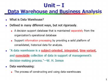
• What is Data Warehouse?
• Defined in many different ways, but not
  rigorously.
• A decision support database that is maintained
  separately from the organizations operational
  database
• Support information processing by providing a
  solid platform of consolidated, historical data
  for analysis.
• A data warehouse is a subject-oriented,
  integrated, time-variant, and nonvolatile
  collection of data in support of managements
  decision-making process.W. H. Inmon
• Data warehousing
• The process of constructing and using data
  warehouses

2
Data WarehouseSubject-Oriented

• Organized around major subjects, such as
  customer, product, sales
• Focusing on the modeling and analysis of data for
  decision makers, not on daily operations or
  transaction processing
• Provide a simple and concise view around
  particular subject issues by excluding data that
  are not useful in the decision support process

3
Data WarehouseIntegrated

• Constructed by integrating multiple,
  heterogeneous data sources
• relational databases, flat files, on-line
  transaction records
• Data cleaning and data integration techniques are
  applied.
• Ensure consistency in naming conventions,
  encoding structures, attribute measures, etc.
  among different data sources
• E.g., Hotel price currency, tax, breakfast
  covered, etc.
• When data is moved to the warehouse, it is
  converted.

4
Data WarehouseTime Variant

• The time horizon for the data warehouse is
  significantly longer than that of operational
  systems
• Operational database current value data
• Data warehouse data provide information from a
  historical perspective (e.g., past 5-10 years)
• Every key structure in the data warehouse
• Contains an element of time, explicitly or
  implicitly
• But the key of operational data may or may not
  contain time element

5
Data WarehouseNonvolatile

• A physically separate store of data transformed
  from the operational environment
• Operational update of data does not occur in the
  data warehouse environment
• Does not require transaction processing,
  recovery, and concurrency control mechanisms
• Requires only two operations in data accessing
• initial loading of data and access of data

6
Data Warehouse vs. Heterogeneous DBMS

• Traditional heterogeneous DB integration A query
  driven approach
• Build wrappers/mediators on top of heterogeneous
  databases
• When a query is posed to a client site, a
  meta-dictionary is used to translate the query
  into queries appropriate for individual
  heterogeneous sites involved, and the results are
  integrated into a global answer set
• Complex information filtering, compete for
  resources
• Data warehouse update-driven, high performance
• Information from heterogeneous sources is
  integrated in advance and stored in warehouses
  for direct query and analysis

7
Data Warehouse vs. Operational DBMS

• OLTP (on-line transaction processing)
• Major task of traditional relational DBMS
• Day-to-day operations purchasing, inventory,
  banking, manufacturing, payroll, registration,
  accounting, etc.
• OLAP (on-line analytical processing)
• Major task of data warehouse system
• Data analysis and decision making
• Distinct features (OLTP vs. OLAP)
• User and system orientation customer vs. market
• Data contents current, detailed vs. historical,
  consolidated
• Database design ER application vs. star
  subject
• View current, local vs. evolutionary, integrated
• Access patterns update vs. read-only but complex
  queries

8
OLTP vs. OLAP
9
Why Separate Data Warehouse?

• High performance for both systems
• DBMS tuned for OLTP access methods, indexing,
  concurrency control, recovery
• Warehousetuned for OLAP complex OLAP queries,
  multidimensional view, consolidation
• Different functions and different data
• missing data Decision support requires
  historical data which operational DBs do not
  typically maintain
• data consolidation DS requires consolidation
  (aggregation, summarization) of data from
  heterogeneous sources
• data quality different sources typically use
  inconsistent data representations, codes and
  formats which have to be reconciled
• Note There are more and more systems which
  perform OLAP analysis directly on relational
  databases

10
From Tables and Spreadsheets to Data Cubes

• A data warehouse is based on a multidimensional
  data model which views data in the form of a data
  cube
• A data cube, such as sales, allows data to be
  modeled and viewed in multiple dimensions
• Dimension tables, such as item (item_name, brand,
  type), or time(day, week, month, quarter, year)
• Fact table contains measures (such as
  dollars_sold) and keys to each of the related
  dimension tables
• In data warehousing literature, an n-D base cube
  is called a base cuboid. The top most 0-D cuboid,
  which holds the highest-level of summarization,
  is called the apex cuboid. The lattice of
  cuboids forms a data cube.

11
Chapter 3 Data Generalization, Data Warehousing,
and On-line Analytical Processing

• Data generalization and concept description
• Data warehouse Basic concept
• Data warehouse modeling Data cube and OLAP
• Data warehouse architecture
• Data warehouse implementation
• From data warehousing to data mining

12
Cube A Lattice of Cuboids
time,item
time,item,location
time, item, location, supplier
13
Conceptual Modeling of Data Warehouses

• Modeling data warehouses dimensions measures
• Star schema A fact table in the middle connected
  to a set of dimension tables
• Snowflake schema A refinement of star schema
  where some dimensional hierarchy is normalized
  into a set of smaller dimension tables, forming a
  shape similar to snowflake
• Fact constellations Multiple fact tables share
  dimension tables, viewed as a collection of
  stars, therefore called galaxy schema or fact
  constellation

14
Example of Star Schema

Sales Fact Table
time_key
item_key
branch_key
location_key
units_sold
dollars_sold
avg_sales
Measures
15
Example of Snowflake Schema
Sales Fact Table
time_key
item_key
branch_key
location_key
units_sold
dollars_sold
avg_sales
Measures
16
Example of Fact Constellation
Shipping Fact Table
time_key
Sales Fact Table
item_key
time_key
shipper_key
item_key
from_location
branch_key
to_location
location_key
dollars_cost
units_sold
units_shipped
dollars_sold
avg_sales
Measures
17
Cube Definition Syntax (BNF) in DMQL

• Cube Definition (Fact Table)
• define cube ltcube_namegt ltdimension_listgt
  ltmeasure_listgt
• Dimension Definition (Dimension Table)
• define dimension ltdimension_namegt as
  (ltattribute_or_subdimension_listgt)
• Special Case (Shared Dimension Tables)
• First time as cube definition
• define dimension ltdimension_namegt as
  ltdimension_name_first_timegt in cube
  ltcube_name_first_timegt

18
Defining Star Schema in DMQL

• define cube sales_star time, item, branch,
  location
• dollars_sold sum(sales_in_dollars), avg_sales
  avg(sales_in_dollars), units_sold count()
• define dimension time as (time_key, day,
  day_of_week, month, quarter, year)
• define dimension item as (item_key, item_name,
  brand, type, supplier_type)
• define dimension branch as (branch_key,
  branch_name, branch_type)
• define dimension location as (location_key,
  street, city, province_or_state, country)

19
Defining Snowflake Schema in DMQL

• define cube sales_snowflake time, item, branch,
  location
• dollars_sold sum(sales_in_dollars), avg_sales
  avg(sales_in_dollars), units_sold count()
• define dimension time as (time_key, day,
  day_of_week, month, quarter, year)
• define dimension item as (item_key, item_name,
  brand, type, supplier(supplier_key,
  supplier_type))
• define dimension branch as (branch_key,
  branch_name, branch_type)
• define dimension location as (location_key,
  street, city(city_key, province_or_state,
  country))

20
Defining Fact Constellation in DMQL

• define cube sales time, item, branch, location
• dollars_sold sum(sales_in_dollars), avg_sales
  avg(sales_in_dollars), units_sold count()
• define dimension time as (time_key, day,
  day_of_week, month, quarter, year)
• define dimension item as (item_key, item_name,
  brand, type, supplier_type)
• define dimension branch as (branch_key,
  branch_name, branch_type)
• define dimension location as (location_key,
  street, city, province_or_state, country)
• define cube shipping time, item, shipper,
  from_location, to_location
• dollar_cost sum(cost_in_dollars), unit_shipped
  count()
• define dimension time as time in cube sales
• define dimension item as item in cube sales
• define dimension shipper as (shipper_key,
  shipper_name, location as location in cube sales,
  shipper_type)
• define dimension from_location as location in
  cube sales
• define dimension to_location as location in cube
  sales

21
Measures of Data Cube Three Categories

• Distributive if the result derived by applying
  the function to n aggregate values is the same as
  that derived by applying the function on all the
  data without partitioning
• E.g., count(), sum(), min(), max()
• Algebraic if it can be computed by an algebraic
  function with M arguments (where M is a bounded
  integer), each of which is obtained by applying a
  distributive aggregate function
• E.g., avg(), min_N(), standard_deviation()
• Holistic if there is no constant bound on the
  storage size needed to describe a subaggregate.
• E.g., median(), mode(), rank()

22
A Concept Hierarchy Dimension (location)
all
all
Europe
North_America
...
region
Mexico
Canada
Spain
Germany
...
...
country
Vancouver
...
...
Toronto
Frankfurt
city
M. Wind
L. Chan
...
office
23
Multidimensional Data

• Sales volume as a function of product, month, and
  region

Dimensions Product, Location, Time Hierarchical
summarization paths
Region
Industry Region Year Category
Country Quarter Product City Month
Week Office Day
Product
Month
24
A Sample Data Cube
Total annual sales of TV in U.S.A.
25
Cuboids Corresponding to the Cube
all
0-D(apex) cuboid
country
product
date
1-D cuboids
product,date
product,country
date, country
2-D cuboids
3-D(base) cuboid
product, date, country
26
Typical OLAP Operations

• Roll up (drill-up) summarize data
• by climbing up hierarchy or by dimension
  reduction
• Drill down (roll down) reverse of roll-up
• from higher level summary to lower level summary
  or detailed data, or introducing new dimensions
• Slice and dice project and select
• Pivot (rotate)
• reorient the cube, visualization, 3D to series of
  2D planes
• Other operations
• drill across involving (across) more than one
  fact table
• drill through through the bottom level of the
  cube to its back-end relational tables (using SQL)

27
Fig. 3.10 Typical OLAP Operations
28
Design of Data Warehouse A Business Analysis
Framework

• Four views regarding the design of a data
  warehouse
• Top-down view
• allows selection of the relevant information
  necessary for the data warehouse
• Data source view
• exposes the information being captured, stored,
  and managed by operational systems
• Data warehouse view
• consists of fact tables and dimension tables
• Business query view
• sees the perspectives of data in the warehouse
  from the view of end-user

29
Data Warehouse Design Process

• Top-down, bottom-up approaches or a combination
  of both
• Top-down Starts with overall design and planning
  (mature)
• Bottom-up Starts with experiments and prototypes
  (rapid)
• From software engineering point of view
• Waterfall structured and systematic analysis at
  each step before proceeding to the next
• Spiral rapid generation of increasingly
  functional systems, short turn around time, quick
  turn around
• Typical data warehouse design process
• Choose a business process to model, e.g., orders,
  invoices, etc.
• Choose the grain (atomic level of data) of the
  business process
• Choose the dimensions that will apply to each
  fact table record
• Choose the measure that will populate each fact
  table record

30
Data Warehouse A Multi-Tiered Architecture
Monitor Integrator
OLAP Server
Metadata
Analysis Query Reports Data mining
Serve
Data Warehouse
Data Marts
Data Sources
OLAP Engine
Front-End Tools
Data Storage
31
Three Data Warehouse Models

• Enterprise warehouse
• collects all of the information about subjects
  spanning the entire organization
• Data Mart
• a subset of corporate-wide data that is of value
  to a specific groups of users. Its scope is
  confined to specific, selected groups, such as
  marketing data mart
• Independent vs. dependent (directly from
  warehouse) data mart
• Virtual warehouse
• A set of views over operational databases
• Only some of the possible summary views may be
  materialized

32
Data Warehouse Development A Recommended Approach
Multi-Tier Data Warehouse
Distributed Data Marts
Enterprise Data Warehouse
Data Mart
Data Mart
Model refinement
Model refinement
Define a high-level corporate data model
33
Data Warehouse Back-End Tools and Utilities

• Data extraction
• get data from multiple, heterogeneous, and
  external sources
• Data cleaning
• detect errors in the data and rectify them when
  possible
• Data transformation
• convert data from legacy or host format to
  warehouse format
• Load
• sort, summarize, consolidate, compute views,
  check integrity, and build indicies and
  partitions
• Refresh
• propagate the updates from the data sources to
  the warehouse

34
Metadata Repository

• Meta data is the data defining warehouse objects.
  It stores
• Description of the structure of the data
  warehouse
• schema, view, dimensions, hierarchies, derived
  data defn, data mart locations and contents
• Operational meta-data
• data lineage (history of migrated data and
  transformation path), currency of data (active,
  archived, or purged), monitoring information
  (warehouse usage statistics, error reports, audit
  trails)
• The algorithms used for summarization
• The mapping from operational environment to the
  data warehouse
• Data related to system performance
• warehouse schema, view and derived data
  definitions
• Business data
• business terms and definitions, ownership of
  data, charging policies

35
OLAP Server Architectures

• Relational OLAP (ROLAP)
• Use relational or extended-relational DBMS to
  store and manage warehouse data and OLAP middle
  ware
• Include optimization of DBMS backend,
  implementation of aggregation navigation logic,
  and additional tools and services
• Greater scalability
• Multidimensional OLAP (MOLAP)
• Sparse array-based multidimensional storage
  engine
• Fast indexing to pre-computed summarized data
• Hybrid OLAP (HOLAP) (e.g., Microsoft SQLServer)
• Flexibility, e.g., low level relational,
  high-level array
• Specialized SQL servers (e.g., Redbricks)
• Specialized support for SQL queries over
  star/snowflake schemas

36
Efficient Data Cube Computation

• Data cube can be viewed as a lattice of cuboids
• The bottom-most cuboid is the base cuboid
• The top-most cuboid (apex) contains only one cell
• How many cuboids in an n-dimensional cube with L
  levels?
• Materialization of data cube
• Materialize every (cuboid) (full
  materialization), none (no materialization), or
  some (partial materialization)
• Selection of which cuboids to materialize
• Based on size, sharing, access frequency, etc.

37
Data warehouse Implementation

• Efficient Cube Computation
• Efficient Indexing
• Efficient Processing of OLAP Queries

38
Cube Operation

• Cube definition and computation in DMQL
• define cube salesitem, city, year
  sum(sales_in_dollars)
• compute cube sales
• Transform it into a SQL-like language (with a new
  operator cube by, introduced by Gray et al.96)
• SELECT item, city, year, SUM (amount)
• FROM SALES
• CUBE BY item, city, year
• Need compute the following Group-Bys
• (date, product, customer),
• (date,product),(date, customer), (product,
  customer),
• (date), (product), (customer)
• ()

39
Multi-Way Array Aggregation

• Array-based bottom-up algorithm
• Using multi-dimensional chunks
• No direct tuple comparisons
• Simultaneous aggregation on multiple dimensions
• Intermediate aggregate values are re-used for
  computing ancestor cuboids
• Cannot do Apriori pruning No iceberg optimization

40
Multi-way Array Aggregation for Cube Computation
(MOLAP)

• Partition arrays into chunks (a small subcube
  which fits in memory).
• Compressed sparse array addressing (chunk_id,
  offset)
• Compute aggregates in multiway by visiting cube
  cells in the order which minimizes the of times
  to visit each cell, and reduces memory access and
  storage cost.

What is the best traversing order to do multi-way
aggregation?
41
Multi-way Array Aggregation for Cube Computation
B
42
Multi-way Array Aggregation for Cube Computation
C
64
63
62
61
c3
c2
48
47
46
45
c1
29
30
31
32
c 0
B
60
13
14
15
16
b3
44
28
B
56
9
b2
40
24
52
5
b1
36
20
1
2
3
4
b0
a1
a0
a2
a3
A
43
Multi-Way Array Aggregation for Cube Computation
(Cont.)

• Method the planes should be sorted and computed
  according to their size in ascending order
• Idea keep the smallest plane in the main memory,
  fetch and compute only one chunk at a time for
  the largest plane
• Limitation of the method computing well only for
  a small number of dimensions
• If there are a large number of dimensions,
  top-down computation and iceberg cube
  computation methods can be explored

44
Indexing OLAP Data Bitmap Index

• Index on a particular column
• Each value in the column has a bit vector bit-op
  is fast
• The length of the bit vector of records in the
  base table
• The i-th bit is set if the i-th row of the base
  table has the value for the indexed column
• not suitable for high cardinality domains

Base table
Index on Region
Index on Type
45
Indexing OLAP Data Join Indices

• Join index JI(R-id, S-id) where R (R-id, ) ?? S
  (S-id, )
• Traditional indices map the values to a list of
  record ids
• It materializes relational join in JI file and
  speeds up relational join
• In data warehouses, join index relates the values
  of the dimensions of a start schema to rows in
  the fact table.
• E.g. fact table Sales and two dimensions city
  and product
• A join index on city maintains for each distinct
  city a list of R-IDs of the tuples recording the
  Sales in the city
• Join indices can span multiple dimensions

46
Efficient Processing OLAP Queries

• Determine which operations should be performed on
  the available cuboids
• Transform drill, roll, etc. into corresponding
  SQL and/or OLAP operations, e.g., dice
  selection projection
• Determine which materialized cuboid(s) should be
  selected for OLAP op.
• Let the query to be processed be on brand,
  province_or_state with the condition year
  2004, and there are 4 materialized cuboids
  available
• 1) year, item_name, city
• 2) year, brand, country
• 3) year, brand, province_or_state
• 4) item_name, province_or_state where year
  2004
• Which should be selected to process the query?
• Explore indexing structures and compressed vs.
  dense array structs in MOLAP

47
Data Warehouse Usage

• Three kinds of data warehouse applications
• Information processing
• supports querying, basic statistical analysis,
  and reporting using crosstabs, tables, charts and
  graphs
• Analytical processing
• multidimensional analysis of data warehouse data
• supports basic OLAP operations, slice-dice,
  drilling, pivoting
• Data mining
• knowledge discovery from hidden patterns
• supports associations, constructing analytical
  models, performing classification and prediction,
  and presenting the mining results using
  visualization tools

48
From On-Line Analytical Processing (OLAP) to On
Line Analytical Mining (OLAM)

• Why online analytical mining?
• High quality of data in data warehouses
• DW contains integrated, consistent, cleaned data
• Available information processing structure
  surrounding data warehouses
• ODBC, OLEDB, Web accessing, service facilities,
  reporting and OLAP tools
• OLAP-based exploratory data analysis
• Mining with drilling, dicing, pivoting, etc.
• On-line selection of data mining functions
• Integration and swapping of multiple mining
  functions, algorithms, and tasks

49
An OLAM System Architecture
Layer4 User Interface
Mining query
Mining result
User GUI API
OLAM Engine
OLAP Engine
Layer3 OLAP/OLAM
Data Cube API
Layer2 MDDB
MDDB
Meta Data
Database API
FilteringIntegration
Filtering
Layer1 Data Repository
Data Warehouse
Data cleaning
Databases
Data integration
50
Chapter 1. Introduction

• Motivation Why data mining?
• What is data mining?
• Data Mining On what kind of data?
• Data mining functionality
• Major issues in data mining

51
Why Data Mining?

• The Explosive Growth of Data from terabytes to
  petabytes
• Data collection and data availability
• Automated data collection tools, database
  systems, Web, computerized society
• Major sources of abundant data
• Business Web, e-commerce, transactions, stocks,
  
• Science Remote sensing, bioinformatics,
  scientific simulation,
• Society and everyone news, digital cameras,
  YouTube
• We are drowning in data, but starving for
  knowledge!
• Necessity is the mother of inventionData
  miningAutomated analysis of massive data sets

52
Evolution of Database Technology

• 1960s
• Data collection, database creation, IMS and
  network DBMS
• 1970s
• Relational data model, relational DBMS
  implementation
• 1980s
• RDBMS, advanced data models (extended-relational,
  OO, deductive, etc.)
• Application-oriented DBMS (spatial, scientific,
  engineering, etc.)
• 1990s
• Data mining, data warehousing, multimedia
  databases, and Web databases
• 2000s
• Stream data management and mining
• Data mining and its applications
• Web technology (XML, data integration) and global
  information systems

53
What Is Data Mining?

• Data mining (knowledge discovery from data)
• Extraction of interesting (non-trivial, implicit,
  previously unknown and potentially useful)
  patterns or knowledge from huge amount of data
• Data mining a misnomer?
• Alternative names
• Knowledge discovery (mining) in databases (KDD),
  knowledge extraction, data/pattern analysis, data
  archeology, data dredging, information
  harvesting, business intelligence, etc.
• Watch out Is everything data mining?
• Simple search and query processing
• (Deductive) expert systems

54
Knowledge Discovery (KDD) Process
Knowledge

• Data miningcore of knowledge discovery process

Pattern Evaluation
Data Mining
Task-relevant Data
Selection
Data Warehouse
Data Cleaning
Data Integration
Databases
55
KDD Process Several Key Steps

• Learning the application domain
• relevant prior knowledge and goals of application
• Creating a target data set data selection
• Data cleaning and preprocessing (may take 60 of
  effort!)
• Data reduction and transformation
• Find useful features, dimensionality/variable
  reduction, invariant representation
• Choosing functions of data mining
• summarization, classification, regression,
  association, clustering
• Choosing the mining algorithm(s)
• Data mining search for patterns of interest
• Pattern evaluation and knowledge presentation
• visualization, transformation, removing redundant
  patterns, etc.
• Use of discovered knowledge

56
Data Mining and Business Intelligence
Increasing potential to support business decisions
End User
Decision Making
Business Analyst
Data Presentation
Visualization Techniques
Data Mining
Data Analyst
Information Discovery
Data Exploration
Statistical Summary, Querying, and Reporting
Data Preprocessing/Integration, Data Warehouses
DBA
Data Sources
Paper, Files, Web documents, Scientific
experiments, Database Systems
57
Data Mining Confluence of Multiple Disciplines
58
Why Not Traditional Data Analysis?

• Tremendous amount of data
• Algorithms must be highly scalable to handle such
  as tera-bytes of data
• High-dimensionality of data
• Micro-array may have tens of thousands of
  dimensions
• High complexity of data
• Data streams and sensor data
• Time-series data, temporal data, sequence data
• Structure data, graphs, social networks and
  multi-linked data
• Heterogeneous databases and legacy databases
• Spatial, spatiotemporal, multimedia, text and Web
  data
• Software programs, scientific simulations
• New and sophisticated applications

59
Multi-Dimensional View of Data Mining

• Data to be mined
• Relational, data warehouse, transactional,
  stream, object-oriented/relational, active,
  spatial, time-series, text, multi-media,
  heterogeneous, legacy, WWW
• Knowledge to be mined
• Characterization, discrimination, association,
  classification, clustering, trend/deviation,
  outlier analysis, etc.
• Multiple/integrated functions and mining at
  multiple levels
• Techniques utilized
• Database-oriented, data warehouse (OLAP), machine
  learning, statistics, visualization, etc.
• Applications adapted
• Retail, telecommunication, banking, fraud
  analysis, bio-data mining, stock market analysis,
  text mining, Web mining, etc.

60
Data Mining Classification Schemes

• General functionality
• Descriptive data mining
• Predictive data mining
• Different views lead to different classifications
• Data view Kinds of data to be mined
• Knowledge view Kinds of knowledge to be
  discovered
• Method view Kinds of techniques utilized
• Application view Kinds of applications adapted

61
Data Mining On What Kinds of Data?

• Database-oriented data sets and applications
• Relational database, data warehouse,
  transactional database
• Advanced data sets and advanced applications
• Data streams and sensor data
• Time-series data, temporal data, sequence data
  (incl. bio-sequences)
• Structure data, graphs, social networks and
  multi-linked data
• Object-relational databases
• Heterogeneous databases and legacy databases
• Spatial data and spatiotemporal data
• Multimedia database
• Text databases
• The World-Wide Web

62
Data Mining Functionalities

• Multidimensional concept description
  Characterization and discrimination
• Generalize, summarize, and contrast data
  characteristics, e.g., dry vs. wet regions
• Frequent patterns, association, correlation vs.
  causality
• Diaper ? Beer 0.5, 75 (Correlation or
  causality?)
• Classification and prediction
• Construct models (functions) that describe and
  distinguish classes or concepts for future
  prediction
• E.g., classify countries based on (climate), or
  classify cars based on (gas mileage)
• Predict some unknown or missing numerical values

63
Data Mining Functionalities (2)

• Cluster analysis
• Class label is unknown Group data to form new
  classes, e.g., cluster houses to find
  distribution patterns
• Maximizing intra-class similarity minimizing
  interclass similarity
• Outlier analysis
• Outlier Data object that does not comply with
  the general behavior of the data
• Noise or exception? Useful in fraud detection,
  rare events analysis
• Trend and evolution analysis
• Trend and deviation e.g., regression analysis
• Sequential pattern mining e.g., digital camera ?
  large SD memory
• Periodicity analysis
• Similarity-based analysis
• Other pattern-directed or statistical analyses

64
Major Issues in Data Mining

• Mining methodology
• Mining different kinds of knowledge from diverse
  data types, e.g., bio, stream, Web
• Performance efficiency, effectiveness, and
  scalability
• Pattern evaluation the interestingness problem
• Incorporation of background knowledge
• Handling noise and incomplete data
• Parallel, distributed and incremental mining
  methods
• Integration of the discovered knowledge with
  existing one knowledge fusion
• User interaction
• Data mining query languages and ad-hoc mining
• Expression and visualization of data mining
  results
• Interactive mining of knowledge at multiple
  levels of abstraction
• Applications and social impacts
• Domain-specific data mining invisible data
  mining
• Protection of data security, integrity, and
  privacy

65
Are All the Discovered Patterns Interesting?

• Data mining may generate thousands of patterns
  Not all of them are interesting
• Suggested approach Human-centered, query-based,
  focused mining
• Interestingness measures
• A pattern is interesting if it is easily
  understood by humans, valid on new or test data
  with some degree of certainty, potentially
  useful, novel, or validates some hypothesis that
  a user seeks to confirm
• Objective vs. subjective interestingness measures
• Objective based on statistics and structures of
  patterns, e.g., support, confidence, etc.
• Subjective based on users belief in the data,
  e.g., unexpectedness, novelty, actionability, etc.

66
Find All and Only Interesting Patterns?

• Find all the interesting patterns Completeness
• Can a data mining system find all the interesting
  patterns? Do we need to find all of the
  interesting patterns?
• Heuristic vs. exhaustive search
• Association vs. classification vs. clustering
• Search for only interesting patterns An
  optimization problem
• Can a data mining system find only the
  interesting patterns?
• Approaches
• First general all the patterns and then filter
  out the uninteresting ones
• Generate only the interesting patternsmining
  query optimization

67
Why Data Mining Query Language?

• Automated vs. query-driven?
• Finding all the patterns autonomously in a
  database?unrealistic because the patterns could
  be too many but uninteresting
• Data mining should be an interactive process
• User directs what to be mined
• Users must be provided with a set of primitives
  to be used to communicate with the data mining
  system
• Incorporating these primitives in a data mining
  query language
• More flexible user interaction
• Foundation for design of graphical user interface
• Standardization of data mining industry and
  practice

68
Primitives that Define a Data Mining Task

• Task-relevant data
• Database or data warehouse name
• Database tables or data warehouse cubes
• Condition for data selection
• Relevant attributes or dimensions
• Data grouping criteria
• Type of knowledge to be mined
• Characterization, discrimination, association,
  classification, prediction, clustering, outlier
  analysis, other data mining tasks
• Background knowledge
• Pattern interestingness measurements
• Visualization/presentation of discovered patterns

69
Primitive 3 Background Knowledge

• A typical kind of background knowledge Concept
  hierarchies
• Schema hierarchy
• E.g., street lt city lt province_or_state lt country
• Set-grouping hierarchy
• E.g., 20-39 young, 40-59 middle_aged
• Operation-derived hierarchy
• email address hagonzal_at_cs.uiuc.edu
• login-name lt department lt university lt country
• Rule-based hierarchy
• low_profit_margin (X) lt price(X, P1) and cost
  (X, P2) and (P1 - P2) lt 50

70
Primitive 4 Pattern Interestingness Measure

• Simplicity
• e.g., (association) rule length, (decision) tree
  size
• Certainty
• e.g., confidence, P(AB) (A and B)/ (B),
  classification reliability or accuracy, certainty
  factor, rule strength, rule quality,
  discriminating weight, etc.
• Utility
• potential usefulness, e.g., support
  (association), noise threshold (description)
• Novelty
• not previously known, surprising (used to remove
  redundant rules, e.g., Illinois vs. Champaign
  rule implication support ratio)

71
Primitive 5 Presentation of Discovered Patterns

• Different backgrounds/usages may require
  different forms of representation
• E.g., rules, tables, crosstabs, pie/bar chart,
  etc.
• Concept hierarchy is also important
• Discovered knowledge might be more understandable
  when represented at high level of abstraction
• Interactive drill up/down, pivoting, slicing and
  dicing provide different perspectives to data
• Different kinds of knowledge require different
  representation association, classification,
  clustering, etc.

72
DMQLA Data Mining Query Language

• Motivation
• A DMQL can provide the ability to support ad-hoc
  and interactive data mining
• By providing a standardized language like SQL
• Hope to achieve a similar effect like that SQL
  has on relational database
• Foundation for system development and evolution
• Facilitate information exchange, technology
  transfer, commercialization and wide acceptance
• Design
• DMQL is designed with the primitives described
  earlier

73
An Example Query in DMQL
74
Other Data Mining Languages Standardization
Efforts

• Association rule language specifications
• MSQL (Imielinski Virmani99)
• MineRule (Meo Psaila and Ceri96)
• Query flocks based on Datalog syntax (Tsur et
  al98)
• OLEDB for DM (Microsoft2000) and recently DMX
  (Microsoft SQLServer 2005)
• Based on OLE, OLE DB, OLE DB for OLAP, C
• Integrating DBMS, data warehouse and data mining
• DMML (Data Mining Mark-up Language) by DMG
  (www.dmg.org)
• Providing a platform and process structure for
  effective data mining
• Emphasizing on deploying data mining technology
  to solve business problems

75
Integration of Data Mining and Data Warehousing

• Data mining systems, DBMS, Data warehouse systems
  coupling
• No coupling, loose-coupling, semi-tight-coupling,
  tight-coupling
• On-line analytical mining data
• integration of mining and OLAP technologies
• Interactive mining multi-level knowledge
• Necessity of mining knowledge and patterns at
  different levels of abstraction by
  drilling/rolling, pivoting, slicing/dicing, etc.
• Integration of multiple mining functions
• Characterized classification, first clustering
  and then association

76
Coupling Data Mining with DB/DW Systems

• No couplingflat file processing, not recommended
• Loose coupling
• Fetching data from DB/DW
• Semi-tight couplingenhanced DM performance
• Provide efficient implement a few data mining
  primitives in a DB/DW system, e.g., sorting,
  indexing, aggregation, histogram analysis,
  multiway join, precomputation of some stat
  functions
• Tight couplingA uniform information processing
  environment
• DM is smoothly integrated into a DB/DW system,
  mining query is optimized based on mining query,
  indexing, query processing methods, etc.

77
Architecture Typical Data Mining System
78
UNIT II- Data Preprocessing

• Data cleaning
• Data integration and transformation
• Data reduction
• Summary

79
Major Tasks in Data Preprocessing

• Data cleaning
• Fill in missing values, smooth noisy data,
  identify or remove outliers, and resolve
  inconsistencies
• Data integration
• Integration of multiple databases, data cubes, or
  files
• Data transformation
• Normalization and aggregation
• Data reduction
• Obtains reduced representation in volume but
  produces the same or similar analytical results
• Data discretization part of data reduction, of
  particular importance for numerical data

80
Data Cleaning

• No quality data, no quality mining results!
• Quality decisions must be based on quality data
• e.g., duplicate or missing data may cause
  incorrect or even misleading statistics
• Data cleaning is the number one problem in data
  warehousingDCI survey
• Data extraction, cleaning, and transformation
  comprises the majority of the work of building a
  data warehouse
• Data cleaning tasks
• Fill in missing values
• Identify outliers and smooth out noisy data
• Correct inconsistent data
• Resolve redundancy caused by data integration

81
Data in the Real World Is Dirty

• incomplete lacking attribute values, lacking
  certain attributes of interest, or containing
  only aggregate data
• e.g., occupation (missing data)
• noisy containing noise, errors, or outliers
• e.g., Salary-10 (an error)
• inconsistent containing discrepancies in codes
  or names, e.g.,
• Age42 Birthday03/07/1997
• Was rating 1,2,3, now rating A, B, C
• discrepancy between duplicate records

82
Why Is Data Dirty?

• Incomplete data may come from
• Not applicable data value when collected
• Different considerations between the time when
  the data was collected and when it is analyzed.
• Human/hardware/software problems
• Noisy data (incorrect values) may come from
• Faulty data collection instruments
• Human or computer error at data entry
• Errors in data transmission
• Inconsistent data may come from
• Different data sources
• Functional dependency violation (e.g., modify
  some linked data)
• Duplicate records also need data cleaning

83
Multi-Dimensional Measure of Data Quality

• A well-accepted multidimensional view
• Accuracy
• Completeness
• Consistency
• Timeliness
• Believability
• Value added
• Interpretability
• Accessibility
• Broad categories
• Intrinsic, contextual, representational, and
  accessibility

84
Missing Data

• Data is not always available
• E.g., many tuples have no recorded value for
  several attributes, such as customer income in
  sales data
• Missing data may be due to
• equipment malfunction
• inconsistent with other recorded data and thus
  deleted
• data not entered due to misunderstanding
• certain data may not be considered important at
  the time of entry
• not register history or changes of the data
• Missing data may need to be inferred

85
How to Handle Missing Data?

• Ignore the tuple usually done when class label
  is missing (when doing classification)not
  effective when the of missing values per
  attribute varies considerably
• Fill in the missing value manually tedious
  infeasible?
• Fill in it automatically with
• a global constant e.g., unknown, a new
  class?!
• the attribute mean
• the attribute mean for all samples belonging to
  the same class smarter
• the most probable value inference-based such as
  Bayesian formula or decision tree

86
Noisy Data

• Noise random error or variance in a measured
  variable
• Incorrect attribute values may due to
• faulty data collection instruments
• data entry problems
• data transmission problems
• technology limitation
• inconsistency in naming convention
• Other data problems which requires data cleaning
• duplicate records
• incomplete data
• inconsistent data

87
How to Handle Noisy Data?

• Binning
• first sort data and partition into
  (equal-frequency) bins
• then one can smooth by bin means, smooth by bin
  median, smooth by bin boundaries, etc.
• Regression
• smooth by fitting the data into regression
  functions
• Clustering
• detect and remove outliers
• Combined computer and human inspection
• detect suspicious values and check by human
  (e.g., deal with possible outliers)

88
Simple Discretization Methods Binning

• Equal-width (distance) partitioning
• Divides the range into N intervals of equal size
  uniform grid
• if A and B are the lowest and highest values of
  the attribute, the width of intervals will be W
  (B A)/N.
• The most straightforward, but outliers may
  dominate presentation
• Skewed data is not handled well
• Equal-depth (frequency) partitioning
• Divides the range into N intervals, each
  containing approximately same number of samples
• Good data scaling
• Managing categorical attributes can be tricky

89
Binning Methods for Data Smoothing

• Sorted data for price (in dollars) 4, 8, 9, 15,
  21, 21, 24, 25, 26, 28, 29, 34
• Partition into equal-frequency (equi-depth)
  bins
• - Bin 1 4, 8, 9, 15
• - Bin 2 21, 21, 24, 25
• - Bin 3 26, 28, 29, 34
• Smoothing by bin means
• - Bin 1 9, 9, 9, 9
• - Bin 2 23, 23, 23, 23
• - Bin 3 29, 29, 29, 29
• Smoothing by bin boundaries
• - Bin 1 4, 4, 4, 15
• - Bin 2 21, 21, 25, 25
• - Bin 3 26, 26, 26, 34

90
Regression
y
Y1
y x 1
Y1
x
X1
91
Cluster Analysis
92
Data Cleaning as a Process

• Data discrepancy detection
• Use metadata (e.g., domain, range, dependency,
  distribution)
• Check field overloading
• Check uniqueness rule, consecutive rule and null
  rule
• Use commercial tools
• Data scrubbing use simple domain knowledge
  (e.g., postal code, spell-check) to detect errors
  and make corrections
• Data auditing by analyzing data to discover
  rules and relationship to detect violators (e.g.,
  correlation and clustering to find outliers)
• Data migration and integration
• Data migration tools allow transformations to be
  specified
• ETL (Extraction/Transformation/Loading) tools
  allow users to specify transformations through a
  graphical user interface
• Integration of the two processes
• Iterative and interactive (e.g., Potters Wheels)

93
Data Integration

• Data integration
• Combines data from multiple sources into a
  coherent store
• Schema integration e.g., A.cust-id ? B.cust-
• Integrate metadata from different sources
• Entity identification problem
• Identify real world entities from multiple data
  sources, e.g., Bill Clinton William Clinton
• Detecting and resolving data value conflicts
• For the same real world entity, attribute values
  from different sources are different
• Possible reasons different representations,
  different scales, e.g., metric vs. British units

94
Handling Redundancy in Data Integration

• Redundant data occur often when integration of
  multiple databases
• Object identification The same attribute or
  object may have different names in different
  databases
• Derivable data One attribute may be a derived
  attribute in another table, e.g., annual revenue
• Redundant attributes may be able to be detected
  by correlation analysis
• Careful integration of the data from multiple
  sources may help reduce/avoid redundancies and
  inconsistencies and improve mining speed and
  quality

95
Correlation Analysis (Numerical Data)

• Correlation coefficient (also called Pearsons
  product moment coefficient)
• where n is the number of tuples, and
  are the respective means of p and q, sp and sq
  are the respective standard deviation of p and q,
  and S(pq) is the sum of the pq cross-product.
• If rp,q gt 0, p and q are positively correlated
  (ps values increase as qs). The higher, the
  stronger correlation.
• rp,q 0 independent rpq lt 0 negatively
  correlated

96
Correlation (viewed as linear relationship)

• Correlation measures the linear relationship
  between objects
• To compute correlation, we standardize data
  objects, p and q, and then take their dot product

97
Data Transformation

• A function that maps the entire set of values of
  a given attribute to a new set of replacement
  values s.t. each old value can be identified with
  one of the new values
• Methods
• Smoothing Remove noise from data
• Aggregation Summarization, data cube
  construction
• Generalization Concept hierarchy climbing
• Normalization Scaled to fall within a small,
  specified range
• min-max normalization
• z-score normalization
• normalization by decimal scaling
• Attribute/feature construction
• New attributes constructed from the given ones

98
Data Transformation Normalization

• Min-max normalization to new_minA, new_maxA
• Ex. Let income range 12,000 to 98,000
  normalized to 0.0, 1.0. Then 73,000 is mapped
  to
• Z-score normalization (µ mean, s standard
  deviation)
• Ex. Let µ 54,000, s 16,000. Then
• Normalization by decimal scaling

Where j is the smallest integer such that
Max(?) lt 1
99
Data Reduction Strategies

• Why data reduction?
• A database/data warehouse may store terabytes of
  data
• Complex data analysis/mining may take a very long
  time to run on the complete data set
• Data reduction Obtain a reduced representation
  of the data set that is much smaller in volume
  but yet produce the same (or almost the same)
  analytical results
• Data reduction strategies
• Dimensionality reduction e.g., remove
  unimportant attributes
• Numerosity reduction (some simply call it Data
  Reduction)
• Data cub aggregation
• Data compression
• Regression
• Discretization (and concept hierarchy generation)

100
Dimensionality Reduction

• Curse of dimensionality
• When dimensionality increases, data becomes
  increasingly sparse
• Density and distance between points, which is
  critical to clustering, outlier analysis, becomes
  less meaningful
• The possible combinations of subspaces will grow
  exponentially
• Dimensionality reduction
• Avoid the curse of dimensionality
• Help eliminate irrelevant features and reduce
  noise
• Reduce time and space required in data mining
• Allow easier visualization
• Dimensionality reduction techniques
• Principal component analysis
• Singular value decomposition
• Supervised and nonlinear techniques (e.g.,
  feature selection)

101
Dimensionality Reduction Principal Component
Analysis (PCA)

• Find a projection that captures the largest
  amount of variation in data
• Find the eigenvectors of the covariance matrix,
  and these eigenvectors define the new space

102
Principal Component Analysis (Steps)

• Given N data vectors from n-dimensions, find k
  n orthogonal vectors (principal components) that
  can be best used to represent data
• Normalize input data Each attribute falls within
  the same range
• Compute k orthonormal (unit) vectors, i.e.,
  principal components
• Each input data (vector) is a linear combination
  of the k principal component vectors
• The principal components are sorted in order of
  decreasing significance or strength
• Since the components are sorted, the size of the
  data can be reduced by eliminating the weak
  components, i.e., those with low variance (i.e.,
  using the strongest principal components, it is
  possible to reconstruct a good approximation of
  the original data)
• Works for numeric data only

103
Feature Subset Selection

• Another way to reduce dimensionality of data
• Redundant features
• duplicate much or all of the information
  contained in one or more other attributes
• E.g., purchase price of a product and the amount
  of sales tax paid
• Irrelevant features
• contain no information that is useful for the
  data mining task at hand
• E.g., students' ID is often irrelevant to the
  task of predicting students' GPA

104
Heuristic Search in Feature Selection

• There are 2d possible feature combinations of d
  features
• Typical heuristic feature selection methods
• Best single features under the feature
  independence assumption choose by significance
  tests
• Best step-wise feature selection
• The best single-feature is picked first
• Then next best feature condition to the first,
  ...
• Step-wise feature elimination
• Repeatedly eliminate the worst feature
• Best combined feature selection and elimination
• Optimal branch and bound
• Use feature elimination and backtracking

105
Feature Creation

• Create new attributes that can capture the
  important information in a data set much more
  efficiently than the original attributes
• Three general methodologies
• Feature extraction
• domain-specific
• Mapping data to new space (see data reduction)
• E.g., Fourier transformation, wavelet
  transformation
• Feature construction
• Combining features
• Data discretization

106
Mapping Data to a New Space

• Fourier transform
• Wavelet transform

Two Sine Waves
Two Sine Waves Noise
Frequency
107
Numerosity (Data) Reduction

• Reduce data volume by choosing alternative,
  smaller forms of data representation