Dead reckoning

1
Dead reckoning
2
In order to determine the actual, current pose,
we use the measured sequence of wheel rotations
(dead reckoning and later additional
information such as vision in a process called
estimation).

• Even if the trajectory is planned as per the
  previous discussion it is important to be able to
  use real-time information to update the actual
  pose.
• We begin with a discussion of the use of
  wheel-rotation information only to accomplish
  this A procedure called dead reckoning.

3
There are three ways that are (nominally)
equivalent to achieve the dead reckoning with our
tricycle example.
4
The first of these entails sampling of wheel
rotations of the two rear wheels only.
5
This makes use of the same kinematics equations
developed for the wheel chair and it requires
knowledge of the dimension 2b.
6
This makes use of the same kinematics equations
developed for the wheel chair and it requires
knowledge of the dimension 2b.
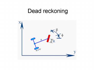
7
The second of these entails the sampling of the
forward rotation a together with the steering
angle b of the single drive/steer wheel.
8
The second of these entails the sampling of the
forward rotation a together with the steering
angle b of the single drive/steer wheel.
9
The second of these entails the sampling of the
forward rotation a together with the steering
angle b of the single drive/steer wheel.
10
Recall that ds can be found from this information
according to dsRdacosb.
11
Recall that ds can be found from this information
according to ds R da cosb.
12
Recall that ds can be found from this information
according to ds R da cosb.
13
Recall that ds can be found from this information
according to ds R da cosb.
14
The third approach is similar. However, it
entails calculation of ds by way of the average
rotation of the two rear wheels, ds r
(dq1dq2)/2
15
The third approach is similar. However, it
entails calculation of ds by way of the average
rotation of the two rear wheels, ds r
(dq1dq2)/2
16
But it also uses the steering angle b as the
basis for calculating u.
17
0.1050 0.0950 -0.09967 0.05025
0.1099 0.0901 -0.19547 0.05024
0.1148 0.0852 -0.28778 0.05097
0.1195 0.0805 -0.37186 0.05367
0.1240 0.0760 -0.44752 0.05546
0.1282 0.0718 -0.51353 0.05740

• If the odometry data, including steering angle,
  are all available, we have a choice of how to
  proceed.

Dq1 Dq2 b
Da
18
0.1050 0.0950 -0.09967 0.05025
0.1099 0.0901 -0.19547 0.05024
0.1148 0.0852 -0.28778 0.05097
0.1195 0.0805 -0.37186 0.05367
0.1240 0.0760 -0.44752 0.05546
0.1282 0.0718 -0.51353 0.05740
Dq1 Dq2 b
Da
19
0.1050 0.0950 -0.09967 0.05025
0.1099 0.0901 -0.19547 0.05024
0.1148 0.0852 -0.28778 0.05097
0.1195 0.0805 -0.37186 0.05367
0.1240 0.0760 -0.44752 0.05546
0.1282 0.0718 -0.51353 0.05740
Dq1 Dq2 b
Da
20
0.1050 0.0950 -0.09967 0.05025
0.1099 0.0901 -0.19547 0.05024
0.1148 0.0852 -0.28778 0.05097
0.1195 0.0805 -0.37186 0.05367
0.1240 0.0760 -0.44752 0.05546
0.1282 0.0718 -0.51353 0.05740
Dq1 Dq2 b
Da
21
0.1050 0.0950 -0.09967 0.05025
0.1099 0.0901 -0.19547 0.05024
0.1148 0.0852 -0.28778 0.05097
0.1195 0.0805 -0.37186 0.05367
0.1240 0.0760 -0.44752 0.05546
0.1282 0.0718 -0.51353 0.05740
Dq1 Dq2 b
Da
22
0.1050 0.0950 -0.09967 0.05025
0.1099 0.0901 -0.19547 0.05024
0.1148 0.0852 -0.28778 0.05097
0.1195 0.0805 -0.37186 0.05367
0.1240 0.0760 -0.44752 0.05546
0.1282 0.0718 -0.51353 0.05740
Dq1 Dq2 b
Da
23
0.1050 0.0950 -0.09967 0.05025
0.1099 0.0901 -0.19547 0.05024
0.1148 0.0852 -0.28778 0.05097
0.1195 0.0805 -0.37186 0.05367
0.1240 0.0760 -0.44752 0.05546
0.1282 0.0718 -0.51353 0.05740

• Lets consider first the use of rotation from the
  two rear wheels.

Dq1 Dq2 b
Da
24
0.1050 0.0950 0.1099 0.0901
0.1148 0.0852 0.1195 0.0805 0.1240
0.0760 0.1282 0.0718 0.1322
0.0678 0.1359 0.0641 0.1392 0.0608
0.1421 0.0579
Dq1 Dq2

• Recall the odometry equations for the wheelchair
• df/daRu/b
• dx/daRcosf
• dy/daRsinf

25
0.1050 0.0950 0.1099 0.0901
0.1148 0.0852 0.1195 0.0805 0.1240
0.0760 0.1282 0.0718 0.1322
0.0678 0.1359 0.0641 0.1392 0.0608
0.1421 0.0579
Dq1 Dq2

• df/daRu/b
• dx/daRcosf
• dy/daRsinf

26
0.1050 0.0950 0.1099 0.0901
0.1148 0.0852 0.1195 0.0805 0.1240
0.0760 0.1282 0.0718 0.1322
0.0678 0.1359 0.0641 0.1392 0.0608
0.1421 0.0579
Dq1 Dq2
27
0.1050 0.0950 0.1099 0.0901
0.1148 0.0852 0.1195 0.0805 0.1240
0.0760 0.1282 0.0718 0.1322
0.0678 0.1359 0.0641 0.1392 0.0608
0.1421 0.0579
Dq1 Dq2
28
0.1050 0.0950 0.1099 0.0901
0.1148 0.0852 0.1195 0.0805 0.1240
0.0760 0.1282 0.0718 0.1322
0.0678 0.1359 0.0641 0.1392 0.0608
0.1421 0.0579
Dq1 Dq2
29
0.1050 0.0950 0.1099 0.0901
0.1148 0.0852 0.1195 0.0805 0.1240
0.0760 0.1282 0.0718 0.1322
0.0678 0.1359 0.0641 0.1392 0.0608
0.1421 0.0579
Dq1 Dq2
30
0.1050 0.0950 0.1099 0.0901
0.1148 0.0852 0.1195 0.0805 0.1240
0.0760 0.1282 0.0718 0.1322
0.0678 0.1359 0.0641 0.1392 0.0608
0.1421 0.0579
Dq1 Dq2
31
0.1050 0.0950 0.1099 0.0901
0.1148 0.0852 0.1195 0.0805 0.1240
0.0760 0.1282 0.0718 0.1322
0.0678 0.1359 0.0641 0.1392 0.0608
0.1421 0.0579
Dq1 Dq2
32
0.1050 0.0950 0.1099 0.0901
0.1148 0.0852 0.1195 0.0805 0.1240
0.0760 0.1282 0.0718 0.1322
0.0678 0.1359 0.0641 0.1392 0.0608
0.1421 0.0579
Dq1 Dq2
33
0.1050 0.0950 0.1099 0.0901
0.1148 0.0852 0.1195 0.0805 0.1240
0.0760 0.1282 0.0718 0.1322
0.0678 0.1359 0.0641 0.1392 0.0608
0.1421 0.0579
Dq1 Dq2

• df/daRu/b
• dx/daRcosf
• dy/daRsinf

34
0.1050 0.0950 0.1099 0.0901
0.1148 0.0852 0.1195 0.0805 0.1240
0.0760 0.1282 0.0718 0.1322
0.0678 0.1359 0.0641 0.1392 0.0608
0.1421 0.0579
Dq1 Dq2

• df/daRu/b
• dx/daRcosf
• dy/daRsinf

35
0.1050 0.0950 0.1099 0.0901
0.1148 0.0852 0.1195 0.0805 0.1240
0.0760 0.1282 0.0718 0.1322
0.0678 0.1359 0.0641 0.1392 0.0608
0.1421 0.0579
Dq1 Dq2

• df/daRu/b
• dx/daRcosf
• dy/daRsinf

36
0.1050 0.0950 0.1099 0.0901
0.1148 0.0852 0.1195 0.0805 0.1240
0.0760 0.1282 0.0718 0.1322
0.0678 0.1359 0.0641 0.1392 0.0608
0.1421 0.0579
Dq1 Dq2

• df/daRu/b
• dx/daRcosf
• dy/daRsinf

37
0.1050 0.0950 0.1099 0.0901
0.1148 0.0852 0.1195 0.0805 0.1240
0.0760 0.1282 0.0718 0.1322
0.0678 0.1359 0.0641 0.1392 0.0608
0.1421 0.0579
Dq1 Dq2

• df/daRu/b
• dx/daRcosf
• dy/daRsinf

38
0.1050 0.0950 0.1099 0.0901
0.1148 0.0852 0.1195 0.0805 0.1240
0.0760 0.1282 0.0718 0.1322
0.0678 0.1359 0.0641 0.1392 0.0608
0.1421 0.0579
Dq1 Dq2

• df/daRu/b
• dx/daRcosf
• dy/daRsinf

39
0.1050 0.0950 0.1099 0.0901
0.1148 0.0852 0.1195 0.0805 0.1240
0.0760 0.1282 0.0718 0.1322
0.0678 0.1359 0.0641 0.1392 0.0608
0.1421 0.0579
Dq1 Dq2

• df/daRu/b
• dx/daRcosf
• dy/daRsinf

40
0.1050 0.0950 0.1099 0.0901
0.1148 0.0852 0.1195 0.0805 0.1240
0.0760 0.1282 0.0718 0.1322
0.0678 0.1359 0.0641 0.1392 0.0608
0.1421 0.0579
Dq1 Dq2

• df/daRu/b
• dx/daRcosf
• dy/daRsinf

41
0.1050 0.0950 0.1099 0.0901
0.1148 0.0852 0.1195 0.0805 0.1240
0.0760 0.1282 0.0718 0.1322
0.0678 0.1359 0.0641 0.1392 0.0608
0.1421 0.0579
Dq1 Dq2

• df/daRu/b
• dx/daRcosf
• dy/daRsinf

42
0.1050 0.0950 0.1099 0.0901
0.1148 0.0852 0.1195 0.0805 0.1240
0.0760 0.1282 0.0718 0.1322
0.0678 0.1359 0.0641 0.1392 0.0608
0.1421 0.0579
Dq1 Dq2

• df/daRu/b
• dx/daRcosf
• dy/daRsinf

43
0.1050 0.0950 0.1099 0.0901
0.1148 0.0852 0.1195 0.0805 0.1240
0.0760 0.1282 0.0718 0.1322
0.0678 0.1359 0.0641 0.1392 0.0608
0.1421 0.0579
Dq1 Dq2

• df/daRu/b
• dx/daRcosf
• dy/daRsinf

44
0.1050 0.0950 0.1099 0.0901
0.1148 0.0852 0.1195 0.0805 0.1240
0.0760 0.1282 0.0718 0.1322
0.0678 0.1359 0.0641 0.1392 0.0608
0.1421 0.0579
Dq1 Dq2

• df/daRu/b
• dx/daRcosf
• dy/daRsinf

45
0.1050 0.0950 -0.09967 0.05025
0.1099 0.0901 -0.19547 0.05024
0.1148 0.0852 -0.28778 0.05097
0.1195 0.0805 -0.37186 0.05367
0.1240 0.0760 -0.44752 0.05546
0.1282 0.0718 -0.51353 0.05740
Dq1 Dq2 b
Da
46
0.1050 0.0950 -0.09967 0.05025
0.1099 0.0901 -0.19547 0.05024
0.1148 0.0852 -0.28778 0.05097
0.1195 0.0805 -0.37186 0.05367
0.1240 0.0760 -0.44752 0.05546
0.1282 0.0718 -0.51353 0.05740
Dq1 Dq2 b
Da
47
0.1050 0.0950 -0.09967 0.05025
0.1099 0.0901 -0.19547 0.05024
0.1148 0.0852 -0.28778 0.05097
0.1195 0.0805 -0.37186 0.05367
0.1240 0.0760 -0.44752 0.05546
0.1282 0.0718 -0.51353 0.05740
Dq1 Dq2 b
Da
48
0.1050 0.0950 -0.09967 0.05025
0.1099 0.0901 -0.19547 0.05024
0.1148 0.0852 -0.28778 0.05097
0.1195 0.0805 -0.37186 0.05367
0.1240 0.0760 -0.44752 0.05546
0.1282 0.0718 -0.51353 0.05740
Dq1 Dq2 b
Da
49
(No Transcript)
50
(No Transcript)
51
Actual Dead-reckoned
52
Actual Dead-reckoned
53
In order to determine the actual, current pose,
we use the measured sequence of wheel rotations
(dead reckoning and later additional
information such as vision in a process called
estimation).

• Even if the trajectory is planned as per the
  previous discussion it is important to be able to
  use real-time information to update the actual
  pose.
• We begin with a discussion of the use of
  wheel-rotation information only to accomplish
  this A procedure called dead reckoning.

54
In order to determine the actual, current pose,
we use the measured sequence of wheel rotations
(dead reckoning and later additional
information such as vision in a process called
estimation).

• More often than not, dead reckoning is
  inadequate we must supplement the odometry
  information with additional samples, external to
  the vehicle.