
Anisotropy, Reversal and Micromagnetics PowerPoint PPT Presentation
1 / 94
Title: Anisotropy, Reversal and Micromagnetics
1
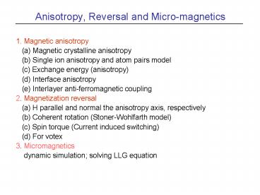
Anisotropy, Reversal and Micro-magnetics
- 1. Magnetic anisotropy
- (a) Magnetic crystalline anisotropy
- (b) Single ion anisotropy and atom pairs model
- (c) Exchange energy (anisotropy)
- (d) Interface anisotropy
- (e) Interlayer anti-ferromagnetic coupling
- 2. Magnetization reversal
- (a) H parallel and normal the anisotropy axis,
respectively - (b) Coherent rotation (Stoner-Wohlfarth model)
- (c) Spin torque (Current induced switching)
- (d) For votex
- 3. Micromagnetics
- dynamic simulation solving LLG equation
2
Magnetocrystalline anisotropy
Crystal structure showing easy and hard
magnetization direction for Fe (a), Ni (b), and
Co (c), above. Respective magnetization curves,
below.
3
(No Transcript)
4
(No Transcript)
5
The Defination of Field Ha
- A quantitative measure of the strength of
the magnetocrystalline anisotropy is the field,
Ha, needed to saturate the magnetization in the
hard direction. - The energy per unit volume needed to
saturate a material in a particular direction is
given by a generation
The uniaxial anisotropy in Co,Ku 1400 x
7000/2 Oe emu/cm3 4.9 x 10⁶ erg/cm3.
6
How is µL coupled to the lattice ?
If the local crystal field seen by an atom is
of low symmetry and if the bonding electrons of
that atom have an asymmetric charge distribution
(Lz ? 0), then the atomic orbits interact
anisotropically with the crystal field. In other
words, certain orientation for the bonding
electron charge distribution are energetically
preferred. The coupling of the spin part of
the magnetic moment to the electronic orbital
shape and orientation (spin-orbit coupling) on a
given atom generates the crystalline anisotropy
7
Physical Origin of Magnetocrystalline anisotropy
Simple representation of the role of orbital
angular momentum ltLzgt and crystalline electric
field in deter- mining the strength of magnetic
anisotropy.
8
(No Transcript)
9
Uniaxial Anisotropy
Careful analysis of the magnetization-orientati
on curves indicates that for most purpose it is
sufficient to keep only the first three terms
where Kuo is independent of the orientation of
M. Ku1gt0 implies an easy axis.
10
- Uniaxial Anisotropy
- Pt/Co or Pd/Co multilayers from interface
- CoCr films from shape
- Single crystal Co in c axis from (magneto-crystal
anisotropy) - MnBi (hcp structure)
- Amorphous GdCo film
- FeNi film
11
Single-Ion Model of Magnetic Anisotropy
de
d?
In a cubic crystal field, the orbital states of
3d electrons are split into two groups one is
the triply degenerate de orbits and the other
the doubly one d ?.
12
Energy levels of deand d d? electrons in (a)
octahedral and (b) tetrahedral sites.
13
Table The ground state and degeneracy of
transition metal ions
14
d electrons for Fe2 in octahe- dral site.
Co2 ions
Oxygen ions
Cations
Distribution of surrounding ions about the
octahedral site of spinel structure.
15
Conclusion
- (1) As for the Fe2 ion, the
sixth electron should occupy the lowest singlet,
so that the ground state is degenerate. - (2) Co2 ion has seven electrons, so that
the last one should occupy the doublet. In such a
case the orbit has the freedom to change its
state in plane which is normal to the trigonal
axis, so that it has an angular momentum parallel
to the trigonal axis. - Since this angular momentum is fixed in
direction, it tends to align the spin magnetic
moment parallel to the trigonal axis through the
spin-orbit interaction.
Slonczewski expalain the stronger anisotropy of
Co2 relative the Fe2 ions in spinel ferrites (
in Magnetism Vol.3, G.Rado and H.Suhl,eds.)
16
Single ion model Ku 2aJ
J(J-1/2)A2ltr2gt, Where A2 is the uniaxial
anisotropy of the crystal field around 4f
electrons, aJ Steven factor, J total anglar
momentum quantum numbee and ltr2gt the average of
the square of the orbital radius of 4f electrons.
Perpendicular anisotropy energy per RE atom
substitution in Gd19Co81films prepared by RF
sputtering (Suzuki at el., IEEE Trans. Magn.
23(1987)2275.
17
over the nearest-neighbor ions j.
18
Y.J.Wang and W.Kleemann PRB 44(1991)5132.
19
References (single ion anisotropy)
- (1) J.J.Rhyne 1972 Magnetic Properties Rare
earth matals ed by R.J.elliott p156 - (2) Z.S.Shan, D.J.Sellmayer, S.S.Jaswal,
Y.J.Wang, and J.X.Shen, - Magnetism of rare-earth tansition metal
nanoscale multilayers, Phys.Rev.Lett.,
63(1989)449 - (3) Y. Suzuki and N. Ohta, Single ion model for
magneto-striction in rare-earth transition metal
amorphous films, J.Appl.Phys., 63(1988)3633 - (4) Y.J.Wang and W.Kleemann,
- Magnetization and perpendicular anisotropy
in Tb/Fe multilayer films, Phys.Rev.B, 44
(1991)5132.
20
Exchange Anisotropy
Co particle 2r20nm
Schematic representation of effect of exchange
coupling on M-H loop for a material with
antiferromagnetic (A) surface layer and a soft
ferro- magnetic layer (F). The anisotropy
field is defined on a hard-axis loop, right (
Meiklejohn and Bean, Phys. Rev. 102(1956)3047 ).
21
FeMn
NiFe
strong-antiferromagnet
weak-antiferromagnete
Above, the interfacial moment configuration in
zero field. Below, left, the weak-antiferromagnete
limit, moments of both films respond in
unison to field. Below, right, in the
strong-antiferromagnet limit, the A moment far
from the interface maintain their orientation.
(Mauri JAP 62(1987)3047)
22
NiFe/FeMn
In the weak-antiferromagnet limit, KA tA
ltlt J, tA ? j / KA tAc, For FeMn system,
tAc 5 0 (A) for j 0.1 mJ/m2 and KA 2x10⁴
mJ/m3.
Exchange field and coecivity as function of
FeMn Thickness (Mauri JAP 62(1987)3047).
23
- Mauri et al., (JAP 62(1987)3047) derived an
expression for - M-H loop of the soft film in the exchange-coupled
regime, (tAgttAc)
There are stable solution at ?0 and
p corresponding to MF.
?
Hex along z direction
24
Interface anisotropy
Carcia et al., APL 47(1985)178
25
(No Transcript)
26
(Si substrate)
Effective anisotropy times Co thickness
versus cobalt thickness for Co/Pt multilayers
(Engle PRL 67(1990)1910).
27
The effective anisotropy energy measured for
a film of thickness d may be described as
(1)
,
or writing as
(2)
(3)
Keff d 2ks (kV -2pMs2)d
28
- Surface Magnetic Anisotropy ?
- The reduced symmetry at the surface (Neel 1954)
- The ratio of Lz2 / (Lx2 Ly2) is increased near
the surface - Interface anisotropy (LS coupling)
1J.G.Gay and Roy Richter, PRL 56(1986)2728, 2
G.H.O. Daalderop et al., PRB 41(1990)11919, 3
D.S.Wang et al., PRL 70(1993)869.
29
Interlayer AF coupling
Grunberg et al., PRL 57(1986)2442
Fe/Cr/Fe Fe/Au/Fe
Fig.2 Spectra from Cr 8 and Au 20 with Bo
along the easy axis. The arrow indicate the
suggested magnetization direction on the two Fe
layers where Bo is supposed to point up. Observed
spin-wave propagation then is along a horizontal
line.
30
Oscillation Exchange Coupling
Field needed to saturate the magnetization at 4.2
K versus Cr thickness for Si(111) / 100ACr /
20AFe / tCr Cr n /50A Cr, deposited at T40oC
( solid circle, N30) at T125oC (open circle,
N20) (Parkin PRL 64 (1990)2304).
31
Interlayer exchange coupling strength J12 for
coupling of Ni80Co20 layers through a Ru spacer
layer. The solid line corresponds to a fit to the
data of RKKY form. Parkin et al., PRB
44(1991)7131.
32
Parkin et al., PRL 66(1991)2152
33
Bruno, Chappert PRL 67(1991)1602
The spin polarization of the conduction electrons
gives rise to an indirect exchange interaction
Hij J(Rij) S i?S j . The interlayer coupling is
obtained by summing Hij over all the pairs ij, i
and j running respectively on F1 and F2.
34
Co/Au(111)/Co
Dependence of the exchange coupling J between
Co layers vs the thickness tAu of the Au(111)
interlayer. Line theoretical fit of experimental
data to RKKY model, with I33.8 erg/cm2, ?4.5
AL, ?0.11 rad, tc5AL and m/m0.16
PRL 71(1993)3023
35
RKKY theory
36
Fermi spanning vector
37
Magnetization Process
- The magnetization process describes the
response of material to applied field. - (1) What does an M-H curve look like ?
- (2) why ?
38
For uniaxial anisotropy and domain walls are
parallel to the easy axis
Application of a field H transverse to the EA
results in rotation of the domain magnetization
but no wall motion. Wall motion appears as H is
parallel to the EA.
39
Hard-Axis Magnetization
The energy density
(1)
(For zero torque condition)
(2)
(For stability condition)
? 0 for H gt 2 Ku / Ms (Ku gt0 )
? the angle between H and M
? p for H lt
-2 Ku / Ms (Ku lt0)
40
- The other solution from eq.1 is given by
(2)
This is the equation of motion for the
magnetization in field below saturation -2Ku/Ms
ltH lt 2Ku/Ms Eq.(2) may be written as
HaMscos? MsH
(3) Using cos?mM/Ms , eq.3 gives
mh,
( hH/Ha)
41
- m h, ( m M/Ms h H/Ha )
It is the general equatiuon for the
magnetization processs with the field applied in
hard direction for an uniaxial material,
M-H loop for hard axis magnetization process
42
M-H loop for easy-axis magnetization process
43
Stoner-Wohlfarth Model
The free energy
f -Kucos2 (?- ?o) HMscos?
Minimizing with respect to ?, giving
Kusin2 (?- ?o) HMssin ?0
Coordinate system for magnetization
reversal process in single-domain particle.
44
Kusin2 (?- ?o) HoMsSin ?0
(1)
?2E/ ? ?2 0 giving,
2KuCos (?- ?o) - Ho MsCos ?0 (2)
Eq.(1) and (2) can be written as sin2(?-
?o) psin? (3)
cos (?- ?o) (p/2)cos? (4)
with pHo Ms/Ku
45
- From eq.(3) and (4) we obtain
(5)
Using Eq.(3-5) one gets
(6)
46
The relationship between p and ?o
Sin2?o(1/p2) (4-p2)/33/2
?o is the angle between H and the easy axis
pHo Ms/Ku.
p
?o 45o, Ho Ku/Ms ?o 0 or 90o, Ho 2Ku/Ms
47
Stoner Wohlfarth model of coherent rotation
Hc 2Ku/Ms
M/Ms
o
H 2Ku/Ms
48
Wall motion coecivity Hc
The change of wall energy per unit area is
H
?ew /? s 2IsHcos ?
? is the angle between H and Is
Ho1/ (2Iscos ?) (?ew/ ?s)max
(1)
49
If the change of wall energy arises from interior
stress
max
(2)
here d is the wall thick. Substitution of (2)
into (1) getting,
When ? d
For common magnet, Homax 200 Oe.
(?10-5, Is1T, so100 KG /mm2.)
50
Ho max p?so/2Iscos?
Dependence of the coercive force on the
magnitude for of internal stress nickel (a)
hard-drawn in various stress (b) a hard-worked
Ni specimen which was an- nealed to release the
internal stress.
51
Coecivity from domain wall pinning
Geometry of medium showing defect region 2 and
host material in regions 1 and 3
Friedburg and Pauil PRL 34(1975)1234.
52
The total energy related to the 180o wall
movement
E?Ai (d?/dx)2 ki sin2? HMi cos ? dx
(1) where i1,2 and 3 in the region 1,2 and
3 respectively Minimizing the total
energy and obtaining the Euler equation -2 Ai
(d2?/dx2 ) 2ki sin?cos ? HMi sin ? 0
(2)
Integrating the Eq.(2) yields the three
nonlinear equations - Ai (d?/dx)2 ki
sin2? - HMi cos? ci (3)
where ci is an integral constant
53
s A(??/ ?z)2dz ds 2A ??? d?/?z?z dz
-2A(? 2?/?z2) d?dz 2A(??/?z)dz
-2A (? 2?/?z2)
54
The boundary condition in the homogeneous
regions is ?(-8)0, ?(8)p, (d ?/dx)x -80,
(d ?/dx)x80, (4) substituting (4) into
(3), one obtains - A (d?/dx)2 - k sin2? -
HMs cos? HMs 0 (5) - A
(d?/dx)2 - k sin2? - HMs cos? - HMs 0
(6) - A (d?/dx)2 - k sin2?- HM2 cos?
c2 (7) they are,
respectively, Euler equations in region of (1),
(3) and (2).
55
Using the continuous condition at
boundary, A d?1.2 / dx A d
?1.2 / dx, one gets
(cos?1 ha/2b)2 (cos?2 ha/2b)2 2h/b
(8) D
A/(AK)1/2 (1-b)sin2?2 -h(1-a)cos?2
bsin2?1 -hacos?1h
-1/2 d?2 (9)
with h HMs / K, a1- M2A/MsA, b1- AK/AK.
When a, b and D are determined, namely the
defects are determined, we can obtain a set of
solution of h, ?1 and ?2, among them there must
be a sets h which is maximun hmax.
56
Solution 1
When the applied field small so as to hlt1,
then eq.9 become D A/(AK)1/2
-cos2 ?2 cos2 ?1/sin2 ?1sin?1
(10) . From eq.(8), cos2 ?1 cos2
?22h/b
(11). Substituting (11) into (10),
we get Hc (KD)/(Msdo)(A/A-K/K
)(sin2 ?1 cos?2)max
(2K / Ms)( D / 32/3do)(A/A- K/K)
(12)
57
Solution 2
If the thickness of the wall is much less
than the thickness of the defect, do ltlt D. In
such a case, the reversal can be performed in
the region 2. Therefore, the contribution from
the region 3 can be ignored for ?2 p. We get
Hc (2K/Ms)(1-pq)(1-(mp)1/2)2/(1-mp)
2 (13) where
pA/A, qK/K, mM2/Ms We see that Hc
is not related to D when do ltlt D
58
w (D/ddw)
- when wltlt1, hc increases lineally with
w
(2) when w is larger, hc is saturated
(3) When Fltlt1 or Eltlt1, larger hc can be
obtained
The normalized Hc vs wall energy of the defect,
EA2K2/A1K1
The normalized Hcvs w (D/ddw)
59
Example-1
Nd2Fe14B
4pMs16 KG, A10-6 erg/cm,
K15x107 erg/cm3 , do 40 A The
Nd2Fe14B grains, 5-10 µm are separated by non
magnetic phase of Nd1.1Fe4B4 and rich-Nd (0.1-1
µm ) and satisfied for wD/do, EF 0
If let F be 0.01, then
hc1.6 or HchcK1M1 40 KOe
60
Example-2
For amorphous alloy, W (D/do) gtgt1 and F 1, E
larger from fig, hc 0.06 is obtained.
Assuming K1 100erg/cm3 and Ms1200 emu/cm3,
then Hc0.006 Oe It
is in agreement with experiment.
61
SST
- L.Berger PRB 54(1996)9353
- 2. J.C.Slonczewski 3M 159(1996)1
62
Spin toque transfer
Tsoi et al PRL 80(1998)4281
Samples (large) (Co/Cu)N MLs N20-50 tCo1.5nm,
tCu2.0-2.2nm capped with 1.6 nm Au Measured at
4.2 K and Jc 109 A/cm2
At negative polarity, current flows from Ag tip
into MLs. H is perpendicular to MLS.
63
H
1200A Cu /100A Co /60A Cu/ 25A Co /150A Cu /30A
Pt/ 600A Au
The device diameter is 130 30 nm
Katine et al PRL 84(2000)3149.
64
At room temperature
J1.0x108 A/cm2
Fig.2 (a) dv/dI of a pillars device exhibits
hysteretic jumps as the current is swept (b)
Zero-bias MR hysteresis loop for the same sample
(Katine PRL 84(2000)3149).
65
g -4(1p)3(3 s1 s2)/4p3/2-1
For I gt Ic a? eS Heff (0) 2pM / g(0)
from parallel to anti-parallel For below Ic-
a? eS Heff (0) -2pM / g(p) from anti-parallel
to parallel
The spin-transfer model predicts that increasing
H should make both Ic and Ic- more positive.
66
Some degree of spin polarization along the
instantaneous axis parallel to the vector s1 of
local ferromagnetic polarization in F1 will be
present in the electrons impinging on F2.
67
spin polarization along the axis parallel to the
vector ML of local ferromagnetic polarization in
will be present in the electrons impinging on
MR. S1,2 (Ieg/c)S1,2 x (S1 x S2)
g -4(1p)3(3S1S2)/4p3/2
(J.C.Slonczwski 3M 159(1996)L1)
68
(No Transcript)
69
The last term incorporates the spin-transfer
effects. The prefactor aI depends on the spin
polarization current p and the angle between the
free and pinned layers (Özyilmaz et al PRL
91(2003)067203).
70
Single-crystal multilayer mad by MBE
25nm(Ga1-xMnx)As/500nm(InyGa1-y)As/100nmGaAs on
(001) semi-insulating GaAs substrate. Sample A
x0.05, y0.15 B x0.038, y0.23 Tc90K for A,
110K for B
Fig 1, A micrograph and a schematic drawing of
the device. (a) a 20 µm wide channel with three
pairs of Hall probes separated by 15 µm was
defined by photolithograhy and wet etching. (b)
to reduce the Hc of two regions, 7-8 nm and 3nm
of the surface layers of regions 2 and 3,
respectively, were removed . A domain wall was
prepared at the boundary of regions 1 and 2, and
its position after application of a current
pulse was monitoredby RHallVHall/l, using a
small probe current I. Voltage VHall is measured
at the Hall probe. Magneto-optical Kerr
microscopy was used to image the domain
structure.
71
Fig 2, The hysteresis loop of regions 1,2 and 3
of sample A measured by RHall at 83K, and the
temperature and the current dependence of the
averaged Hall resis- tance, RHall. (a) Hc shows
that Hc(1)gtHc(3)gtHc(2), as designed. No
dependence of hysteresis on current direction
was observed at I5µA. (b) Temperature
dependence of RHall measured using I5µA, 1.5-s
current pulses open circies Indicate RHall for
region 1, closed triangles for 2, and open
downward triangles for 3. (c) Current dependence
of RHall measured 1.5-s current pulses at 82K.
72
Fig 3, The effect of successive
alternating negative and positive current pulses
on RHall for regions 1,2 and 3 of sample A. The
amplitude of the pulse is 350 µA and its width
100ms. At t0, the domain wall is at the
boundary of regions 1 and 2 when a negative
current pulse is applied (t30s), M direction in
region 2 is reversed. The M direction in region
2 can be switched back.
73
initial state After I-300 µA After I
300 µA
Fig 4, MOKE images of sample A using 546 nm light
at 80K.
74
R.P.Cowburn et al., (Uni Cambridge) PRL
83(1999)1042.
Reversal in votex
75
(No Transcript)
76
(No Transcript)
77
(No Transcript)
78
(No Transcript)
79
Motion Equation for Magnetic vector
There is angle moment G corresponding to M
and the relation between them
M -? G,
(1) under the action of Heff, M is
acted by a torque,
L M x Heff.
(2) Due to the torque,
dG/dt M x Heff,
(3) substituting (1)
to (3), we obtain
dM/dt -? M x Heff,
(4) This is the Motion Equation for
Magnetic vector
80
He
At t1, the position of M is represented by M.
Under the action of He, M is affected by a
torque LM x He and M moves to the position of
M at t2t1dt. As such a manner, M moves
with a constant length and a continuous
variant direction. This behaviors of M is
called as the precession motion of M around He.
t2t1dt.
-L
-L
t2
M
M
t1
o
G
G
81
dM/dt -? M x Heff, which is a motion
equation without any damping. When the damping
term in the equation exits, M is quickly parallel
to the direction of He. The expression of
the damping term (1) Landau-Lifshith form
Td (-a?/M) x M x ( M x Heff), (2)
Gilbert form Td (a/M) M x dM / dt
82
Micromagnetics-Dynamic Simulation
(1) The film is divided into nx ny regular
elements, (2) Determining all the field on each
element
(3) Solving Landau-Lifshith-Gilbert equation
83
Two dimension
Magnetic thin film modelded in two-dimensional
approximation. The film is divided into nx x ny
ele- ments for the simulation.
84
?M lt 1.0 x10⁻⁷ G The sum torque T lt102 erg/cc
Computation flow diagram for solving the
magnetization In the magnetic film.
85
(1) To set the parameters Ms1400 G, Ku1x106
erg/cm3, random anisotropy from 0-180o,
A2x10-6 erg/cm, d20nm, a1 (2) mx(i,j)m
sinTcos ß, my(i,j), mz(i,j) dmx(i,j)0,
dmy(i,j)0 dmz(i,j)0 (3)
mx(i,j)mx(i,j)dmx(i,j), dmy(i,j), dmz(i,j) (4)
? mx(i,j)/N i from 1 to 20, j from 1 to 20
(5) t from 10-3 to 1 sec, dt10-12 (6) To
calculate Hk(i,j), Hd(i,j), Hex(i,j),
Hap(i,j) (7) To solving the LLG eqation (8) To
calculate torque and dm
86
Micromagnetics-dynamic simulation
Cross-tie wall in thin Permalloy film simulated
(a and b) and observed (c) Nakatani et al.,
Japanese JAP 28(1989)2485.
87
Hysterisis Loop Simulation(an example Co/Ru/Co
and Co/Ru/Co/Ru/Co Films)
Co
Ru
Co
Co
Ru
Co
Ru
Co
Wang YJ et al., JAP 89(2001)699491(2002)9241
94(2003)525.
88
Landau-Lifshitz-Gilbert Equation
89
(No Transcript)
90
(No Transcript)
91
The other fields
(1) Random anisotropy field ha ( m e )
hK , m M/Ms , and e denotes the unit
vector along the easy axis in the
cell (2) Exchange energy fild hex
(3) Demagnetizing field (dipole-dipole
interaction) hmagi - ? (1/rij3)
3(mj rij)/rij mj
(4) The applied field happ h m
92
(No Transcript)
93
(No Transcript)
94
Thanks !
Recommended
