
Artificial Neural Networks PowerPoint PPT Presentation
1 / 102
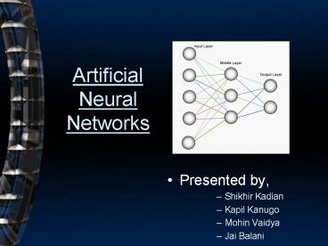
Title: Artificial Neural Networks
1
Artificial Neural Networks
- Presented by,
- Shikhir Kadian
- Kapil Kanugo
- Mohin Vaidya
- Jai Balani
2
References
- http//www.comp.glam.ac.uk/digimaging/neural.htm
- http//www.nbb.cornell.edu/neurobio/linster/lectur
e4.pdf - http//people.arch.usyd.edu.au/rob/applets/neuro/
SelfOrganisingMapDemo.html - http//www.cis.hut.fi/jhollmen/dippa/node23.html
- http//www.ucl.ac.uk/oncology/MicroCore/HTML_resou
rce/SOM_Intro.htm - http//www.ucl.ac.uk/oncology/MicroCore/HTML_resou
rce/SOM_Intro.htm
3
Introduction to Artificial Neural Networks
4
Introduction
- Why ANN?
- Some tasks can be done easily (effortlessly) by
humans but are hard by conventional paradigms on
Von Neumann machine with algorithmic approach - Pattern recognition (old friends, hand-written
characters) - Content addressable recall
- Approximate, common sense reasoning (driving,
playing piano, baseball player) - These tasks are often ill-defined, experience
based, hard to apply logic
5
Introduction
- What is an (artificial) neural network?
- A set of nodes (units, neurons, processing
elements) 1.Each node has input and output - 2.Each node performs a simple computation by
its node function - Weighted connections between nodes
- Connectivity gives the structure/architecture of
the net - What can be computed by a NN is primarily
determined by the connections and their weights
6
Introduction
What can a ANN do?
- Compute a known function
- Approximate an unknown function
- Pattern Recognition
- Signal Processing
- Learn to do any of the above
7
Introduction
Biological neural activity
- Each neuron has a body, an axon, and many
dendrites - Can be in one of the two states firing and rest.
- Neuron fires if the total incoming stimulus
exceeds the threshold - Synapse thin gap between axon of one neuron and
dendrite of another. - Signal exchange
- Synaptic strength/efficiency
8
Introduction
Neurone vs. Node
9
Introduction
Basic Concepts
- Definition of a node
- A node is an element which performs the function
- y fH(?(wixi) Wb)
10
Introduction
Basic Concepts
- A Neural Network generally maps a set of inputs
to a set of outputs - Number of inputs/outputs is variable
- The Network itself is composed of an arbitrary
number of nodes with an arbitrary topology
11
Introduction
Data
Normalization Max-Min normalization formula is as
follows Example we want to normalize data
to range of the interval -1,0. We put
new_maxA 1, new_minA 0.
Say, max A was 80 and min A was 20 ( That means
maximum and minimum values for the attribute
). Now, if v 50 ( If for this particular
pattern , attribute value is 40 ), v will be
calculated as , v (50-20) x (1-0) / (80-20)
0 gt v 30 x 1/60
gt v 0.5
12
Introduction
The artificial neural network
y1 y2 y3 y4
x1 x2 x3 x4
x5
13
Introduction
Feed-forward nets
- Information flow is unidirectional
- Data is presented to Input layer
- Passed on to Hidden Layer
- Passed on to Output layer
- - Information is distributed
- Information processing is parallel
14
Introduction
Recurrent Networks
- Recurrency
- Nodes connect back to other nodes or themselves
- Information flow is multidirectional
- Sense of time and memory of previous state(s)
- Biological nervous systems show high levels of
recurrency (but feed-forward structures exists
too)
15
Backpropagation Algorithm
Introduction
- Training SetA collection of input-output
patterns that are used to train the network - Testing SetA collection of input-output patterns
that are used to assess network performance - Learning Rate-?A scalar parameter, analogous to
step size in numerical integration, used to set
the rate of adjustments
16
Introduction
- Data is presented to the network in the form of
activations in the input layer - Examples
- Pixel intensity (for pictures)
- Molecule concentrations (for artificial nose)
- Share prices (for stock market prediction)
- How to represent more abstract data, e.g. a name?
- Choose a pattern, e.g.
- 0-0-1 for Chris
- 0-1-0 for Becky
17
Introduction
Binary activation function
Given a net input Ij to unit j, then Oj
f(Ij), the output of unit j, is computed as Oj
1 if ljgtT Oj 0 if ljltT Where T is known as
the Threshold
Squashing activation function
Each unit in the hidden and output layers takes
its net input and then applies an activation
function. The function symbolizes the activation
of the neuron represented by the unit. It is also
called a logistic, sigmoid, or squashing
function. Given a net input Ij to unit j, then
Oj f(Ij), the output
of unit j, is computed as
18
Pseudo-Code Algorithm
Introduction
- Randomly choose the initial weights
- While error is too large
- For each training pattern (presented in random
order) - Apply the inputs to the network
- Calculate the output for every neuron from the
input layer, through the hidden layer(s), to the
output layer - Calculate the error at the outputs
- Use the output error to compute error signals for
pre-output layers - Use the error signals to compute weight
adjustments - Apply the weight adjustments
- Periodically evaluate the network performance
19
Introduction
Error Correction
- For supervised learning
- Perceptron learning (Used for binary values)
In the simple McCullock and Pitts Perceptron
model, each neuron calculates a weighted sum of
inputs, then compares the result to a threshold
value. It outputs a 1 if the sum gt the threshold,
otherwise it outputs a zero.
- Perceptron Learning Formula
- ?wi cdi oixi
- So the value of ?wi is either
- 0 (when expected output and actual output are the
same) - Or
- cxi (when di oi is /-1)
20
By Mohin Vaidya
- Neural Networks Algorithms Explanied
21
Hebbian Learning Formula
- A purely feed forward unsupervised learning
network - Hebbian learning formula comes from Hebbs
postulation that if two neurones were very active
at the same time which is illustrated by the high
values of both its output and one of its inputs,
the strength of the connection between the two
neurones will grow or increase.
22
Hebbian Learning Formula
- If xj is the input of the neuron, xi the output
of the neuron, and wij the strength of the
connection between them, and ? learning rate,
then one form of a learning formula would be - ?Wij (t) ?xjxi
23
Hebbian Learning Formula
24
- Example
- Consider a black box neural approach where one
neuron receives input from the airpuff and from
the tone.
25
Application of the hebbian learning rule the
linear associator
26
Existing research can be summarised as follows
- Back-Propagation Algorithm
- Hebbian Learning Based Algorithm
- Vector Quantization Neural Networks
- Predictive Coding Neural Networks.
27
1. Basic Back-Propagation Neural Network for
image compression
28
Coupling weights wji, j 1, 2, ... K and i 1,
2, ... N which can also be described by a matrix
of KN. From the hidden layer to the output
layer, the connections can be represented by
wij which is another weight matrix of NK.
- where xi0, 1 denotes the normalised pixel values
29
With this basic back-propagation neural network,
compression is conducted in two phases
- Training
- This is equivalent to compressing the input into
the narrow channel represented by the hidden
layer and then reconstructing the input from the
hidden to the output layer. - Encoding
- The second phase simply involves the entropy
coding of the state vector hj at the hidden layer.
30
K-L transform technology
- K-L transform technique is a technique for
simplifying a data set, by reducing
multidimensional data sets to lower dimensions
for analysis.
31
What does K-L transform do?The K-L transform
maps input images into a new vector space
- Eigen vectors and eigen values
32
K-L transform or encoding can be defined as
- and the inverse K-L transform or decoding can be
defined as
33
From the comparison between the equation pair
(3-4) and the equation pair (5-6), it can be
concluded that the linear neural network reaches
the optimum solution whenever the following
condition is satisfied
- Under this circumstance, the neurone weights from
input to hidden and from hidden to output can be
described respectively as follows
34
2. Hierarchical Back-Propagation Neural Network
35
3. Adaptive Back-Propagation Neural Network
36
Training of such a neural network can be designed
as
- a) parallel training
- (b) serial training
- (c) activity based training
- Prior to training, all image blocks are
classified into four classes according to their
activity values which are identified as very low,
low, high and very high activities.
37
4. Hebbian Learning Based Image Compression
- The general neural network structure consists of
one input layer and one output layer.
38
5. Vector Quantization Neural Networks
- K-dimensional space.
- M neurones are designed
- The coupling weight, wij, associated with the
ith neurone is eventually trained to represent
the code-word ci. - With this general structure, various learning
algorithms have been designed and developed such
as - Kohonens self-organising feature mapping,
competitive learning, frequency sensitive
competitive learning, fuzzy competitive learning,
general learning, and distortion equalised fuzzy
competitive learning
39
Let Wi(t) be the weight vector of the ith
neurone at the tth iteration, the basic
competitive learning algorithm can be summarised
as follows
- where d(x, Wi(t)) is the distance in L2 metric
between input vector x and the coupling weight
vector Wi(t) wi1, wi2, ... wiK and zi is its
output.
40
Under-utilisation problem
- Kohonen self-organising neural network
- Frequency sensitive competitive learning algorithm
41
6. Predictive Coding Neural Networks
- De-correlating input data
- Linear and non-linear AR models
- With linear AR model, predictive coding can be
described by the following equation
42
Multi-layer perceptron neural network
43
The output of each neurone, say the jth
neurone, can be
derived from the equation given below
44
To predict those drastically changing features
inside images such as edges, contours etc.,
high-order terms are added to improve the
predictive performance. This corresponds to a
non-linear AR model expressed as follows
- Hence, another functional link type neural
network can be designed to implement this type of
non-linear AR model with high-order terms.
45
Predictive Neural Networks
46
Self Organised Maps ANN And Its Applications
Stony Brook University
By Kapil Kanugo
47
SOM Architecture
- Set of neurons / cluster units
- Each neuron is assigned with a prototype vector
that is taken from the input data set - The neurons of the map can be arranged either on
a rectangular or a hexagonal lattice - Every neuron has a neighborhood as shown in the
figure
Hexagonal
Rectangular
48
SOM in Classification
- Initialization
- Training
- Competition
- Cooperation
- Visualization
- Synaptic Adaption
49
Initialization
- Consider an n-dimensional dataset
- Each row in the data set is treated as a
n-dimensional vector - For each neuron /classifier unit in the map
assign a a prototype vector from the data set - Prototype vectors are initialized
- Randomly
- Linearly
- After training Prototype vectors serves as an
exemplar for all the vector that associated with
the neuron
50
Training Best matching procedure
- Let Xi be a neuron in grid
- be the prototype vector associated to
- be a arbitrary vector
- Now our task is to map this x to any one of the
neuron - For each neuron compute the distance
- Better statistic
- Neuron satisfying the above statistic is the
winner and denoted by b - Applying Update Rule for neighborhood of winner
node.
51
Training Topology
- Training and Topology adjustments are made
iteratively until a sufficiently accurate map is
obtained - After training the prototype vectors contain the
cluster means for the classification - Neurons can be labeled with the cluster means or
classes of the associated prototype vectors
52
Self-Organizing Maps
- SOMs Competitive Networks where
- 1 input and 1 output layer.
- All input nodes feed into all output nodes.
- Output layer nodes are NOT a clique. Each node
has a few neighbors. - On each training input, all output nodes that are
within a topological distance, dT, of D from the
winner node will have their incoming weights
modified. - dT(yi,yj) nodes that must be traversed in the
output layer in moving between output nodes yi
and yj. - D is typically decreased as training proceeds.
Output
Input
Input
Partially Intraconnected
Fully Interconnected
Fully Interconnected
53
There Goes The Neighborhood
D 1
D 2
D 3
- As the training period progresses, gradually
decrease D. - Over time, islands form in which the center
represents the centroid C of a set of input
vectors, S, while nearby neighbors represent
slight variations on C and more distant
neighbors are major variations. - These neighbors may only win on a few (or no)
input vectors, while the island center will win
on many of the elements of S.
54
Self Organization
- In the beginning, the Euclidian distance
dE(yl,yk) and Topological distance dT(yl,yk)
between output nodes yl and yk will not be
related. - But during the course of training, they will
become positively correlated Neighbor nodes in
the topology will have similar weight vectors,
and topologically distant nodes will have very
different weight vectors.
Emergent Structure of Output Layer
Euclidean Neighbor
Topological Neighbor
Before
After
55
The Algorithm
56
(No Transcript)
57
(No Transcript)
58
(No Transcript)
59
(No Transcript)
60
(No Transcript)
61
(No Transcript)
62
(No Transcript)
63
(No Transcript)
64
Data Visualization using SOM
- The idea is to visually present many variables
together offering a degree of control over a
number of different visual properties - High dimensionality of data set and visual
properties such as color, size can be added to
the position property for proper visualization
purposes. - Multiple views can be used by linking all
separate views together when the use of these
properties makes it difficult.
65
Case Study Character Recognition
66
Case Study Character Recognition
- Preprocessing
- Illumination
- Spatial Filtering (Mean Filter)
- Thresholding
- Extraction of Strip
- Segmentation
- Calibration
- Identification
67
Overall Mechanism
Binarisation
Preprocessing
Segmentation using heuristic algorithm
Training of Segmentation ANN
Segmentation Validation using ANN
Extraction of individual words
Training of Character Recognizing ANN
68
Steps in Recognition
- Character Identification involves
- Artificial Neural Networks Algorithm
- Training the Network
- Updating using Learning Algorithm
- Iteratively training the network
- Winner Take All Algorithm
69
Thresholding and Filtering
70
Segmented Digits
71
Winner Take all Algorithm
Generate Wm,Itr500
- Neuron with max responseWinner
- Weight is altered using
- wm µ(x-wm)
- Wnew wm wm
- µ Learning Constant(0.1-0.8)
- Number of Iterations gt500
Multiply Wm x IMAGE
Find Index of max value and Modify Wm
using Update rule
Itrlt500
Storage of final matrix
Stop
72
Digit Identification
73
Specimen System
74
Content-based image classification using a
Neural Network Authors Soo Beom Park, Jae Won
Lee and Sang Kyoon Kim Cited By Science Direct,
Volume 25, February 2004, Pages 287-300
Presented By, Jai Balani
75
References
- http//domino.research.ibm.com/comm/research_proje
cts.nsf/pages/marvel.details.html - http//www.research.ibm.com/marvel/details.html
- http//www.sciencedirect.com/science?_obArticleUR
L_udiB6V15-4B3K380-1_user334567_coverDate02
2F292F2004_rdoc1_fmt_origsearch_sortdvie
wc_acctC000017318_version1_urlVersion0_use
rid334567md5980e88d5edab6646ae0245fe0ad5f761 - http//www.sciencedirect.com/science?_obMImg_ima
gekeyB6V15-4B3K380-1-1S_cdi5665_user334567_o
rigsearch_coverDate022F292F2004_sk999749996
viewcwchpdGLbVlb-zSkWbmd551e3bc898b4757e4d9c
6d4432e680bd4ie/sdarticle.pdf - http//www.neurosolutions.com/products/nsmatlab/ap
psum-textureclassification.html
76
"One picture is worth a thousand words - Fred R.
Barnard
Content-based image classification using a Neural
Network
Technology that makes digital photos searchable
through automated tagging of visual content using
Image Indexing and Classification
techniques. The basics Image
Indexing Obtaining the metadata of any
multimedia content file which contains the
content-based description of the file rather than
the context and title of the file.
"Content-based" means that the search will
analyze the actual contents of the image. The
term 'content' in this context might refer
colors, shapes, textures, or any other
information that can be derived form the image
itself. Contd..
77
Contd Image Classification The intent of the
classification process is to categorize all
pixels in a digital image into one of several
land cover classes, or "themes". The objective of
image classification is to identify and portray,
as a unique gray level (or color), the features
occurring in an image in terms of the object or
type of land cover.
Forested lands divided into two level categories,
deciduous and coniferous.
78
Problem Issues with Indexing
- Indexing audio-visual documents relates to five
basic issues - (1) Which audio-visual features to index for a
given application (e.g. the names of the actors,
the spoken words and the scene type for video
footage), - (2) How to extract them (e.g. neural network
classifier for face recognition, spectral
features for speech recognition, etc.) - (3) How to organize the index table. Most of the
scientific works done so far address the second
issue, and most of the time for one modality,
either visual, auditory or textual - (4) Identifying appropriate features to be
encoded relates to a careful analysis of the use
cases with the end users. - (5) Selecting the indexing organization relates
more to a content-based descriptor scheme.
79
Solution The MPEG-7 Standard
- Moving Picture Experts Group or MPEG is a working
group of ISO/IEC charged with the development of
video and audio encoding standards. - MPEG-7 is a multimedia content description
standard, it is formally called Multimedia
Content Description Interface. - Definitions in this context
- Multimedia Image, Video and Audio files.
- Content The actual display or voice
content in the files. - Description Will be associated with the
content itself, to allow fast and
efficient searching for material that is of
interest to the user. - Standard Descriptor (D), Multimedia
Description Schemes (DS), Description
Definition Language (DDL) - Descriptor (D) It is a representation of a
feature defined syntactically and semantically.
It could be that an unique object was described
by several descriptors. - Multimedia Description Schemes (DS) Specify the
structure and semantics of the relations between
its components, these components can be
descriptors (D) or description schemes (DS). - Description Definition Language (DDL) It is
based on XML language used to define the
structural relations between descriptors. It
allows the creation and modification of
description schemes and also the creation of new
descriptors (D).
80
Relation between different tools and elaboration
process of MPEG-7
81
MPEG-7 Objectives
- Provide a fast and efficient searching,
filtering and content identification method. - Describe main issues about the content
(low-level characteristics, structure, - models, collections, etc.).
- Index a big range of applications.
- Audiovisual information that MPEG-7 deals is
- Audio, voice, video, images, graphs and 3D
models - Inform about how objects are combined in a
scene. - Independence between description and the
information itself.
82
MPEG-7 Objectives
- It was designed to standardize a set of
description schemes and descriptors a - language to specify these schemes, called the
Description Definition Language (DDL) - a scheme for coding the description
- Thus, it is not a standard which deals with the
actual encoding of moving pictures and audio,
like MPEG-1, MPEG-2 and MPEG-4. - It uses XML to store metadata, and can be
attached to time code in order to tag particular
events, or synchronize lyrics to a song. - What for
- Manual annotation is costly and inadequate.
- Manual labeling and cataloging is very costly and
time consuming and often subjective, leading to
incomplete and inconsistent annotations and poor
system performance. - More effective methods for searching,
categorizing and organizing multimedia data.
83
Classification of the object image
- Image classifier consists of three modules
- (1) A preprocessing module
- The preprocessing module removes the background
of an image and performs normalization on the
image. - (2) A feature extraction module
- The feature extraction module enables the
acquisition of the shape and texture information
from the image and extracts a structural feature
value. - (3) A classification module
- The classification module creates a learning
pattern and creates a neural network classifier.
84
Classification of the object image
85
Phase1 Preprocessing of Image Removing
Background
- Objective In the preprocessing step we extract
the object region from the - background using a region segmentation
technique. - It involves the following steps
- Image segmentation using the JSEG
- An extraction of core object region
- Object region and background region
classification - The removal of a corner region
- Resizing and normalization of the image size
- Step 1.1 Image segmentation using the JSEG
- The JSEG method, a CBIR system, it is useful to
segment an image independent of texture. This
method uses a J-value to segment the region. The
J-value is the distribution similarity degree of
color and texture. - The first step of the JSEG method quantizes the
input image. It creates a class-map by labeling
the color value quantized and it creates the
J-image according to J-value that reflects the
spatial features. - It continuously creates an image segmented
through growing and merging of the region around
the J-image.
86
Phase1 Preprocessing of Image Removing
Background
An example of the JSEG region segmentation.
87
Phase1 Preprocessing of Image Removing
Background
- Step 1.2 An extraction of core object region
- As the interesting region, we suppose a half
window of the original image, as Figure. From the
regions segmented in this half window, we select
the largest region as the core object region. In
Figure, the region colored black is the extracted
core object region.
Figure Extraction of the core object region.
88
Phase1 Preprocessing of Image Removing
Background
Step 1.3 Object region and background region
classification Successively, a texture feature
value from each region is extracted. To measure
the similarity, the texture feature values of the
core object region are compared with the values
of other regions extracted. The low-similarity
regions are regarded as the background region and
hence removed.
Figure The result of background regions removal.
89
Phase1 Preprocessing of Image Removing
Background
Step 1.4. The removal of a corner region For
more exact removal, we remove all the corner
regions as a background region. We regard it as a
rare occurrence that object regions stretch over
corner regions. Therefore, unconditionally, the
corner regions are removed automatically. Taken
as a whole, we do not care about the minority
error of object region occurred rarely at
corners.
90
Phase1 Preprocessing of Image Removing
Background
Step 1.5. Resizing and normalization of the image
size We extract a structural feature to extract
as much information as possible. But, the size
and position of the object in an image is
various. When extracting the structural feature
values, there is the problem that each of the
feature values is extracted differently according
to the size and position of the object. To solve
this problem, we resize the background-removed
image in order to exclude the unrelated feature
values from these object images. Since the
neural network classifier requires all image data
to be the same size. we normalize the image to be
128 128.
The result of resizing and normalizing (a) the
resized image, (b) the normalized image.
91
Phase2 A feature extraction module
- Step 2.1 Wavelet Transformation
- The wavelet transform classifies the data into
the sub-bands, low and high frequency. Analyzing
the sub-bands created by transformation, we
acquire the images information. - Step 2.2 Conversion of the color model
- We use the intensity of HSI color model that is
derived from the original RGB image. Below given
figure shows the conversion from the RGB color
model to the HSI color model.
In the converted HSI color model, the intensity
is useful because of the reason that it is
isolated from the color information in image,
hence we use the intensity as a substitute for
the color.
92
Phase2 A feature extraction module
- Step 2.3 Texture feature extraction and learning
pattern creation - The elements to express the texture feature
consist of coarseness, contrast, and
directionality. Coarseness means the rough degree
of texture. Contrast means the pitch distribution
of brightness, and directionality means the
specific direction of texture. Using the equation
given below various texture feature values were
acquired for our experiment.
P(i,j) is a pixel value of each image array.
93
Phase2 A classification module
- Neural network classifier using the learning
pattern of the texture feature to reflect a shape
of an object.
The neural network classifier consists of three
layers with an input layer, a hidden layer, and
an output layer. The neural network is trained
and change weights until the minimum error
reduces to 0.1.
The structure of a neural network.
94
Phase2 A classification module
As a neural network learning algorithm, the
multi-layer perceptron is the most usual. It is
the generalized least mean square (LMS) rule, and
it uses the Gradient Search method to minimize
the average difference between the output and the
target value on the neural network.
95
Phase2 A classification module
Problem Definition The problem is to distinguish
between the leopard and the background, in which
it is sitting in the image shown below.
Figure Original Image to be classifed
96
Phase2 A classification module
- Solution
- Sample small 5x5 pixel images from sections of
the image that represent the leopard and sections
that represents the background. - Flatten the sampled 2D images into one-row
vectors and use them as training data for a
neural network.
Sample small 5x5 pixel sub-images that represent
the leopard and the background. Each red square
represents a sub-image of the leopard and each
yellow square represents a sub-image of the
background.
97
Phase2 A classification module
- Solution
- 3. Sampled images are flattened into single rows
vectors. - Example
- one_image 151 150 144 141 144 154 154 151 149
150 155 155 154 153 150 155 156 158 156 150 158
160 164 162 151 - flattened_image
- Columns 1 through 12
- 151 150 144 141 144 154 154 151 149 150 155 155
- Columns 13 through 24
- 154 153 150 155 156 158 156 150 158 160 164 162
- Column 25
- 151
- 4. The one-row vectors are used to train a
neural network - 5. The entire image is sampled as 5x5 sub-images
as before and are flatten into one-row vectors. - 6. The trained neural network is now tested on
all of 5x5 sub images to determine which ones are
part of the leopard and which ones are part of
the background.
98
Phase2 A classification module
Figure 3 The trained neural network's response
indicates which sub-images represent the leopard
and which ones represent the background.The red
squares represent the areas that the neural
network determined to be the leopard.
99
Image Indexing Applications
- There are many applications and application
domains which will benefit from - the Content based Indexing techniques. A few
application examples are - Digital library Image/video catalogue, musical
dictionary. - Multimedia directory services e.g. yellow
pages. - Broadcast media selection Radio channel, TV
channel. - Multimedia editing Personalized electronic news
service, media authoring. - Security services Traffic control, production
chains... - E-business Searching process of products.
- Cultural services Art-galleries, museums...
- Educational applications.
100
Marvel v/s Google Videos
101
(No Transcript)
102
- Thank You
- Have a pleasant Spring Break ?
Recommended
