Zoom Lenses

1
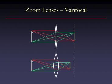
Zoom Lenses Varifocal
2
Zoom Lenses Parfocal
3
Computing Field of View
1/do 1/di 1/f
tan ? /2 ½ xo / do
xo / do xi / di
? 2 tan-1 ½ xi (1/f?1/do)
? ? xi / f
4
Filtering and Edge Detection

5
Local Neighborhoods

• Hard to tell anything from a single pixel
• Example you see a reddish pixel. Is this the
  objects color? Illumination? Noise?
• The next step in order of complexity is to look
  at local neighborhood of a pixel

6
Linear Filters

• Given an image In(x,y) generate anew image
  Out(x,y)
• For each pixel (x,y)Out(x,y) is a linear
  combination of pixelsin the neighborhood of
  In(x,y)
• This algorithm is
• Linear in input intensity
• Shift invariant

7
Discrete Convolution

• This is the discrete analogue of convolution
• The pattern of weights is called the kernel of
  the filter
• Will be useful in smoothing, edge detection

8
Example Smoothing
Original Mandrill
Smoothed withGaussian kernel
9
Gaussian Filters

• One-dimensional Gaussian
• Two-dimensional Gaussian

10
Gaussian Filters
11
Gaussian Filters
12
Gaussian Filters

• Gaussians are used because
• Smooth
• Decay to zero rapidly
• Simple analytic formula
• Limit of applying multiple filters is Gaussian
• Separable G2(x,y) G1(x) G1(y)

13
Computing Convolutions

• What happens near edges of image?
• Ignore (Out is smaller than In)
• Pad with zeros (edges get dark)
• Replicate edge pixels
• Wrap around
• Reflect
• Change filter

14
Computing Convolutions

• If In is n?n, f is m?m, takes time O(m2n2)
• OK for small filter kernels, bad for large ones

15
Digression Fourier Transforms

• Define Fourier transform of function f as
• F is a function of frequency describes how much
  of each frequency f contains
• Fourier transform is invertible

16
Fourier Transform and Convolution

• Fourier transform turns convolutioninto
  multiplication F (f(x) ? g(x)) F (f(x)) F
  (g(x))

17
Fourier Transform and Convolution

• Useful application 1 Use frequency space to
  understand effects of filters
• Example Fourier transform of a Gaussianis a
  Gaussian
• Thus attenuates high frequencies

?

18
Fourier Transform and Convolution

• Useful application 2 Efficient computation
• Fast Fourier Transform (FFT) takes time O(n
  log n)
• Thus, convolution can be performed in time
  O(n log n m log m)
• Greatest efficiency gains for large filters

19
Edge Detection

• What do we mean by edge detection?
• What is an edge?

20
What is an Edge?
21
What is an Edge?
Where is edge? Single pixel wide or multiple
pixels?
22
What is an Edge?
Noise have to distinguish noise from actual edge
23
What is an Edge?
Is this one edge or two?
24
What is an Edge?
Texture discontinuity
25
Formalizing Edge Detection

• Look for strong step edges
• One pixel wide look for maxima in dI / dx
• Noise rejection smooth (with a Gaussian) over a
  neighborhood ?

26
Canny Edge Detector

• Smooth
• Find derivative
• Find maxima
• Threshold

27
Canny Edge Detector

• First, smooth with a Gaussian ofsome width ?

28
Canny Edge Detector

• Next, find derivative
• What is derivative in 2D? Gradient

29
Canny Edge Detector

• Useful fact 1 differentiation commutes with
  convolution
• Useful fact 2 Gaussian is separable

30
Canny Edge Detector

• Thus, combine first two stages of Canny

31
Canny Edge Detector
Original Lena
Smoothed Gradient Magnitude
32
Canny Edge Detector

• Nonmaximum suppression
• Eliminate all but local maxima in magnitudeof
  gradient
• At each pixel look along direction of
  gradientif either neighbor is bigger, set to
  zero
• In practice, quantize direction to horizontal,
  vertical, and two diagonals
• Result thinned edge image

33
Canny Edge Detector

• Final stage thresholding
• Simplest use a single threshold
• Better use two thresholds
• Find chains of edge pixels, all greater than ?
  low
• Each chain must contain at least one pixel
  greater than ? high
• Helps eliminate dropouts in chains, without being
  too susceptible to noise
• Thresholding with hysteresis

34
Canny Edge Detector
Original Lena
Edges
35
Other Edge Detectors

• Can build simpler, faster edge detector by
  omitting some steps
• No nonmaximum suppression
• No hysteresis in thresholding
• Simpler filter

36
Second-Derivative-BasedEdge Detectors

• To find local maxima in derivative, look for
  zeros in second derivative
• Analogue in 2D Laplacian

37
LOG

• As before, combine Laplacian with Gaussian
  smoothing Laplacian of Gaussian (LOG)

38
LOG

• As before, combine Laplacian with Gaussian
  smoothing Laplacian of Gaussian (LOG)

39
Problems withLaplacian Edge Detectors

• Local minimum vs. local maximum
• Symmetric poor performance near corners
• Sensitive to noise along an edge
• Higher-order derivatives greater noise
  sensitivity