Ch 14: From Randomness to Probability Dealing with Random Phenomena

1
Ch 14 From Randomness to Probability Dealing
with Random Phenomena

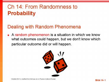
• A random phenomenon is a situation in which we
  know what outcomes could happen, but we dont
  know which particular outcome did or will happen.

2
Probability

• The probability of an event is its long-run
  relative frequency.
• While we may not be able to predict a particular
  individual outcome, we can talk about what will
  happen in the long run.
• For any random phenomenon, each attempt, or
  trial, generates an outcome.
• These outcomes are individual possibilities, like
  the number we see on top when we roll a die.
• Sometimes we are interested in a combination of
  outcomes, called an event
• A die is rolled and comes up even or odd. These
  are both events!
• When thinking about combinations of outcomes,
  things are easiest if the individual trials are
  independent.
• The outcome of one trial doesnt influence or
  change the outcome of another. (e.g. coin tosses,
  die rolls)

3
The Law of Large Numbers

• The Law of Large Numbers (LLN) says that the
  long-run relative frequency of repeated
  independent events gets closer and closer to the
  true relative frequency as the number of trials
  increases.
• Consider flipping a fair coin many, many times.
  The overall percentage of heads should settle
  towards about 50.
• A common misunderstanding of the LLN is that
  random phenomena are supposed to compensate for
  whatever happened in the past. This is not true.
• When flipping a fair coin, if heads comes up on
  each of the first 10 flips, what is the chance it
  will land tails next ?

4
Probability

• Thanks to the LLN, we know that relative
  frequencies settle down in the long run, so we
  can officially give the name probability to that
  value.
• Probabilities must be between 0 and 1, inclusive.
• A probability of 0 indicates impossibility.
• A probability of 1 indicates certainty.

5
Equally Likely Outcomes

• When probability was first studied, a group of
  French mathematicians looked at games of chance
  in which all the possible outcomes were equally
  likely.
• Its equally likely to get any one of six
  outcomes from the roll of a fair die.
• Its equally likely to get heads or tails from
  the toss of a fair coin.
• However, keep in mind that events are not always
  equally likely.
• A skilled basketball player has a better than
  50-50 chance of making a free throw.
• your stats professor has much less than a 50-50
  chance!

6
Personal Probability

• In everyday speech, when we express a degree of
  uncertainty without basing it on long-run
  relative frequencies, we are stating subjective
  or personal probabilities.
• Personal probabilities lack the consistency that
  we need probabilities to have, so well stick
  with formally defined probabilities in this class.

7
Formal Probability

• Two requirements for a probability
• A probability is a number between 0 and 1.
• For any event A, 0 P(A) 1.

8
Formal Probability (cont.)

• Something has to happen rule
• The probability of the set of all possible
  outcomes of a trial must be 1.
• P(S) 1 (S represents the set of all possible
  outcomes.)

9
Formal Probability (cont.)

• Complement Rule
• The set of outcomes that are not in the event A
  is called the complement of A, denoted AC.
• The probability of an event occurring is 1 minus
  the probability that it doesnt occur P(A) 1
  P(AC)

This is a Venn Diagram, which is discussed more
in Chapter 15
10
Formal Probability (cont.)

• Addition Rule
• Events that have no outcomes in common (and,
  thus, cannot occur together) are called disjoint
  (or mutually exclusive).

11
Formal Probability (cont.)

• Addition Rule
• For two disjoint events A and B, the probability
  that one or the other occurs is the sum of the
  probabilities of the two events.
• P(A or B) P(A) P(B), provided that A and B
  are disjoint.

12
Formal Probability (cont.)

• Multiplication Rule
• For two independent events A and B, the
  probability that both A and B occur is the
  product of the probabilities of the two events.
• P(A and B) P(A) x P(B), provided that A and B
  are independent.

• Two independent events A and B are not
  disjoint, provided that each of these events has
  a probability greater than zero

13
Formal Probability (cont.)

• Multiplication Rule- Independence
• Many Statistics methods require an Independence
  Assumption, but assuming independence doesnt
  make it true.
• Always Think about whether that assumption is
  reasonable before using the Multiplication Rule.

14
Formal Probability - Notation

• Notation alert
• In this text we use the notation P(A or B) and
  P(A and B).
• In other situations, you might see the following
• P(A ? B) instead of P(A or B)
• P(A ? B) instead of P(A and B)

15
Putting the Rules to Work

• In most situations where we want to find a
  probability, well use the rules in combination.
• A point to remember is that it can be easier to
  work with the complement of the event were
  really interested in.

16
What Can Go Wrong?

• Beware of probabilities that dont add up to 1.
• To be a legitimate probability distribution, the
  sum of the probabilities for all possible
  outcomes must total 1.
• Dont add probabilities of events if theyre not
  disjoint.
• Events must be disjoint to use the Addition Rule.
• Dont multiply probabilities of events if theyre
  not independent.
• The multiplication of probabilities of events
  that are not independent is one of the most
  common errors people make in dealing with
  probabilities.
• Dont confuse disjoint and independentdisjoint
  events cant be independent.

17
What have we learned?

• Probability is based on long-run relative
  frequencies.
• The Law of Large Numbers speaks only of long-run
  behavior.
• Watch out for misinterpreting the LLN.
• There are some basic rules for combining
  probabilities of outcomes to find probabilities
  of more complex events. We have the
• First check if probabilities for individual
  outcomes make sense
• Then..
• Something Has to Happen Rule
• Complement Rule
• Addition Rule for disjoint events
• Multiplication Rule for independent events
• Also always do a Sanity Check on your results.
  If your calculations give you a probability
  greater than 1 or less than 0, you know youve
  made a mistake!

18
Example

• 11 A consumer organization estimates that over
  a 1 year period, 17 of cars will need to be
  repaired once, 7 will need to be repaired twice
  and 4 will require 3 or more repairs (regardless
  of car make or year, apparently). According to
  this study, what is the probability that a random
  car will need
• No repairs
• No more than 1 repair
• Some repairs

19
Example

• 13 15 Now assume you have 2 cars. Using the
  info from the prior study, what is the
  probability that
• Neither car needs repairs?
• Both will need repairs?
• At least 1 car will need to be repaired?
• What needs to be true about the cars to make this
  approach valid? Is it a reasonable assumption?

20
More Examples

• 24 The American Red Cross says 45 of the US
  population has Type O blood, 40 Type A , 11
  Type B and the rest Type AB (although in reality
  there are other rarer types, we will assume they
  do not exist now).
• If someone has volunteered to give blood, what is
  the probability this donor is
• Type AB
• Has either Type A or Type B
• Is not Type O
• For the next 4 donors that walk in, what is the
  probability that
• They are all Type O
• No one is Type A
• They are all not Type A (note this is different
  than 2b!)
• At least 1 person is Type B?
• What has to be true for us to do this? Is this
  assumption justified?

21
Yet More Examples

• 36 You are drawing cards out of a standard deck
  (52 cards, no jokers) that youve just shuffled.
  The first 10 cards you have drawn are all red.
  You start thinking The next one has got to be
  black
• Are you absolutely correct in your reasoning?
• Is it more likely that you might draw a black
  than red card?
• Compute the probability of drawing
• a red card next.
• a black card next.
• Is this an example of the Law of Large numbers?