Elasticity of Substitution

1
Elasticity of Substitution

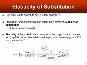
• How easy is it to substitute one input for
  another???
• Production functions may also be classified in
  terms of elasticity of substitution
• Shape of a single isoquant
• Elasticity of Substitution is a measure of the
  proportionate change in K/L (capital to labor
  ratio) relative to the proportionate change in
  MRTS along an isoquant

2
Note Throughout

• Book uses ? for substitution elasticity
• I use s
• They are the same ? s
• It just seems to me that s is used more often in
  the literature.

3
Elasticity of Substitution

• Movement from A to B results in
• L becomes bigger, K becomes smaller
• capital/labor ratio (K/L) decreasing
• MRTS -dK/dL MPL/MPK
• gt MRTSKL decreases
• Along a strictly convex isoquant, K/L and MRTS
  move in same direction
• Elasticity of substitution is positive
• Relative magnitude of this change is measured by
  elasticity of substitution
• If it is high, MRTS will not change much relative
  to K/L and the isoquant will be less curved (less
  strictly convex)
• A low elasticity of substitution gives rather
  sharply curved isoquants

MRTSA
MRTSB
4
Elasticity of Substitution Perfect-Substitute

• ? ?, a perfect-substitute technology
• Analogous to perfect substitutes in consumer
  theory
• A production function representing this
  technology exhibits constant returns to scale
• (?K, ?L) a?K b?L ?(aK bL) ?(K, L)
• All isoquants for this production function are
  parallel straight lines with slopes -b/a

5
Elasticity of substitution for perfect-substitute
technologies
s 8
6
Elasticity of Substitution Leontief

• ? 0, a fixed-proportions (or Leontief )
  technology
• Analogous to perfect complements in consumer
  theory
• Characterized by zero substitution
• A production technology that exhibits fixed
  proportions is

• This production function also exhibits constant
  returns to scale

7
Elasticity of substitution for fixed-proportions
technologies

• Capital and labor must always be used in a fixed
  ratio
• Marginal products are constant and zero
• Violates Monotonicity Axiom and Law of
  Diminishing Marginal Returns
• Isoquants for this technology are right angles gt
  Kinked
• At kink, MRTS is not uniquecan take on an
  infinite number of positive values
• K/L is a constant, d(K/L) 0, which results in ?
  0

s 0
8
Elasticity of Substitution Cobb-Douglas

• ? 1, Cobb-Douglas technology
• Isoquants are strictly convex
• Assumes diminishing MRTS
• An example of a Cobb-Douglas production function
  is
• q (K, L) aKbLd
• a, b, and d are all positive constants
• Useful in many applications because it is linear
  in logs

9
Isoquants for a Cobb-Douglas production function
s 1
10
Constant Elasticity of Substitution (CES)

• ? some positive constant
• Constant elasticity of substitution (CES)
  production function can be specified
• q ??K-? (1 - ?)L- ?-1/?
• ? gt 0, 0 ? 1, ? -1
• ? is efficiency parameter
• ? is a distribution parameter
• ? is substitution parameter
• Elasticity of substitution is
• ? 1/(1 ?)
• Useful in empirical studies

11
Investigating Production

• Spreadsheets available to assess Cobb-Douglas and
  Constant Elasticity of Substitution Production
  Functions.
• On Website
• I suggest reviewing them.

12
Technical Progress/Technological Change
K
Technical Progress shifts the isoquant
inward The same output can be produced with
less/fewer inputs
K0
K1
q0
q1
L1
L0
L
13
How to Measure Technical Progress?

• If q A(t)fK(t), L(t),
• The term A(t) represents factors that influence
  output given levels of capital and labor.
• Proxy for technical progress

14
Technical Progress Continued
Divide result on previous page by q and adjust
Some identities
output elasticity wrt labor eL
output elasticity wrt capital eK
15
Technical Progress Continued
Rate of Growth of Output is

• Rate of Growth of Output is equal to
• Rate of growth of autonomous technological change
• Plus rate of growth of capital times eK (output
  elasticity of capital)
• Plus rate of growth of labor times eL (output
  elasticity of labor)

16
Historically
Data from Robert Solows study of technological
progress in the US, 1909 - 1949
17
Annual Productivity Growth in Agriculture (1965
1994) (Nin et al., 2003)
18
How much can the world produce?

• DICE Model (W. Nordhaus see Nordhaus and Boyer,
  2000).
• Dynamic Integrated Model of Climate and the
  Economy.
• Production
• Q(t) A(t)(K(t)0.30L(t)0.70)
• A(0) 0.018
• K(t) 73.6 trillion
• L(t) 6,484 million (world population)
• Q(t) denominated in trillion/year

19
Additional Assumptions

• A(t) increases at 0.37 per year.
• Global average increase in productivity.
• Compare to alternative 0.19 per year.