4 Postulates of QM

1
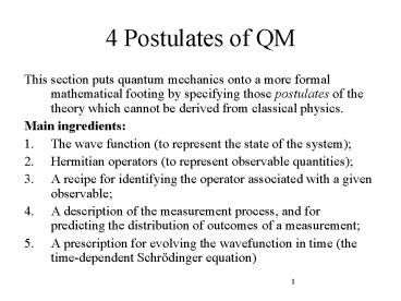
4 Postulates of QM

• This section puts quantum mechanics onto a more
  formal mathematical footing by specifying those
  postulates of the theory which cannot be derived
  from classical physics.
• Main ingredients
• The wave function (to represent the state of the
  system)
• Hermitian operators (to represent observable
  quantities)
• A recipe for identifying the operator associated
  with a given observable
• A description of the measurement process, and for
  predicting the distribution of outcomes of a
  measurement
• A prescription for evolving the wavefunction in
  time (the time-dependent Schrodinger equation)

2
4.1 The wave function
Postulate 4.1 There exists a wavefunction ? that
is a continuous, square-integrable, single-valued
function of the coordinates of all the particles
and of time, and from which all possible
predictions about the physical properties of the
system can be obtained.
Examples of the meaning of The coordinates of
all the particles
x
For a single particle moving in one dimension
Cartesian coordinates
For a single particle moving in three dimensions
or
spherical polar coordinates
For two particles moving in three dimensions
(Cartesian coordinates)
The modulus squared of ? for any value of the
coordinates is the probability density (per unit
length, or volume) that the system is found with
that particular coordinate value (Born
interpretation).
3
4.2 Observables and operators
Postulate 4.2.1 to each observable quantity is
associated a linear, Hermitian operator (LHO).
An operator is linear if and only if
Examples which of the operators defined by the
following equations are linear?
No
Note the operators involved may or may not be
differential operators (i.e. may or may not
involve differentiating the wavefunction).
Yes
No
Yes
4
Hermitian operators
An operator O is Hermitian if and only if
for all functions f, g vanishing at infinity.
Compare the definition of a Hermitian matrix M
Analogous if we identify a matrix element with an
integral
(see 3226 course for more detail)
5
Hermitian operators examples
since x is real ?
??
not Hermitian because of minus sign
?
6
Eigenvectors and eigenfunctions
Postulate 4.2.2 the eigenvalues of the operator
represent the possible results of carrying out a
measurement of the corresponding quantity.
Definition of an eigenvalue for a general linear
operator
Eigenfunction
Operator acting on function Eigenvalue ?
Function
Compare definition of an eigenvalue of a matrix
Matrix ? Vector Eigenvalue ? Vector
Example the time-independent Schrodinger
equation
The energy in the T.I.S.E. is an eigenvalue of
the Hamiltonian operator Interpretation of an
einefunction a state of the system having
adefinite value of the operator (observable)
concerned.
7
Important fact The eigenvalues of a Hermitian
operator are real (like the eigenvalues of a
Hermitian matrix).
is Hermitian
Proof
Let
With
definition of H.O.
RHS
LHS
Is real
LHS RHS
Postulate 4.2.3 immediately after making a
measurement, the wavefunction is identical to an
eigenfunction of the operator corresponding to
the eigenvalue just obtained as the measurement
result.
Ensures that we get the same result if we
immediately re-measure the same quantity.
Start with wavefunction
measure quantity
obtain result
One of the eigenvalues of
Leave system in wavefunction corresponding to
8
4.3 Identifying the operators
Postulate 4.3 the operators representing the
position and momentum of a particle are
(one dimension)
(three dimensions)
or
Other operators may be obtained from the
corresponding classical quantities by making
these replacements.
Examples
The Hamiltonian (representing the total energy as
a function of the coordinates and momenta)
Angular momentum
9
Eigenfunctions of momentum
The momentum operator is Hermitian, as required
Hermitian, despite the fact that
is not Hermitian
Its eigenfunctions are plane waves
10
Orthogonality of eigenfunctions
The eigenfunctions of a Hermitian operator
belonging to different eigenvalues are orthogonal.
then
If
Proof
Use definition of Hermitian operator, taking
11
Orthonormality of eigenfunctions
What if two eigenfunctions have the same
eigenvalue? (In this case the eigenvalue is said
to be degenerate.)
Any linear combination of these eigenfunctions is
also an eigenfunction with the same eigenvalue
So we are free to choose as the eigenfunctions
two linear combinations that are orthogonal.

• Can choose to have all eigenfunctions orthogonal,
  regardless
• of whether eigenvalues are the same or
  different.

If the eigenfunctions are all orthogonal and
normalized, they are said to be orthonormal.
12
Orthonormality of eigenfunctions Example
Consider the solutions of the time-independent
Schrodinger equation (energy eigenfunctions) for
an infinite square well
We chose the constants so that normalization is
correct
Now consider different values of n, m
(i) Two odd values of n
(ii) Two even values of n Try
(iii) Even/odd values
by symmetry
Note
13
Complete sets of functions
The eigenfunctions fn of a Hermitian operator
form a complete set, meaning that any other
function satisfying the same boundary conditions
can be expanded as
If the eigenfunctions are chosen to be
orthonormal, the coefficients an can be
determined as follows
by
and integrate
? To find am, just multiply
We will see the significance of such expansions
when we come to look at the measurement process.
14
Normalization and expansions in complete sets
The condition for normalizing the wavefunction is
now
If the eigenfunctions fn are orthonormal, this
becomes
Natural interpretation the probability of
finding the system in the state fn(x) (as opposed
to any of the other eigenfunctions) is
15
Expansion in complete sets example
Consider an infinite square well, with particle
confined to a ? x ? a
Energy eigenfunction are
So, any function which satisfies the
same boundary conditions(ie, zero outside the
well) can be represented as
with
This is a Fourier series representation of
(Done in maths 2nd year)
16
4.4 Eigenfunctions and measurement
Postulate 4.4 suppose a measurement of the
quantity Q is made, and that the (normalized)
wavefunction can be expanded in terms of the
(normalized) eigenfunctions fn of the
corresponding operator as
Then the probability of obtaining the
corresponding eigenvalue qn as the measurement
result is
Corollary if a system is definitely in
eigenstate fn, the result measuring Q is
definitely the corresponding eigenvalue qn.
What is the meaning of these probabilities in
discussing the properties of a single system?
Still a matter for debate, but usual
interpretation is that the probability of a
particular result determines the frequency of
occurrence of that result in measurements on an
ensemble of similar systems.
17
Commutators
In general operators do not commute that is to
say, the order in which we allow operators to act
on functions matters
For example, for position and momentum operators
We define the commutator as the difference
between the two orderings
Two operators commute only if their commutator is
zero.
So, for position and momentum
Note The commutator of anyoperator with itself
0
ie
18
Compatible operators
Two observables are compatible if their operators
share the same eigenfunctions (but not
necessarily the same eigenvalues).
Consequence two compatible observables can have
precisely-defined values simultaneously.
Measure observable R, definitely obtain result rm
(the corresponding eigenvalue of R)
Measure observable Q, obtain result qm (an
eigenvalue of Q)
Re-measure Q, definitely obtain result qm once
again
Wavefunction of system is corresponding
eigenfunction fm
Wavefunction of system is still corresponding
eigenfunction fm
Compatible operators commute with one another
Expansion in terms of joint eigenfunctions of
both operators
Can also show the converse any two commuting
operators are compatible.
19
Example measurement of position (1)
Eigenfunctions of the position operator x would
be states of definite position. These are the so
called Dirac delta functions that you study in
2nd year maths
For now, consider approximate eigenstates
suppose we have a series of detectors, along a
line, each of which is sensitive to the position
of a particle in a length D. Can expand any
state in terms of efuntions
In n-th region but 0 otherwise. They are
normalised to 1
20
Example measurement of position (2)
Can expand wavefunction as
(becomes exact in limit
)
Where
Probability of finding particle at n-th value of
x
21
Expectation values
The average (mean) value of measurements of the
quantity Q is therefore the sum of the possible
measurement results times the corresponding
probabilities
if
We can also write this as
since
22
4.5 Evolution of the system
Postulate 4.5 Between measurements (i.e. when it
is not disturbed by external influences) the
wave-function evolves with time according to the
time-dependent Schrodinger equation.
Hamiltonian operator.
This is a linear, homogeneous differential
equation, so the linear combination of any two
solutions is also a solution the superposition
principle.
and
if
23
Calculating time dependence using expansion in
energy eigenfunctions
Suppose the Hamiltonian is time-independent. In
that case we know that solutions of the
time-dependent Schrodinger equation exist in the
form
where the wavefunctions ?(x) and the energy E
correspond to one solution of the
time-independent Schrodinger equation
We know that all the functions ?n together form a
complete set, so we can expand
Hence we can find the complete time dependence
(superposition principle)
24
Time-dependent behaviour example
Suppose the state of a particle in an infinite
square well at time t 0 is a superposition of
the n 1 and n 2 states
Wave function at a subsequent time t
Probability density
This is NOT a stationary state since
25
Rate of change of expectation value
Consider the rate of change of the expectation
value of a quantity Q
since
intrinsic time dependence of operator
time dependence from changing wavefunctions
26
Example 1 Conservation of probability
Rate of change of total probability that the
particle may be found at any point
Total probability is the expectation value of
the operator 1.
Total probability conserved (related to existence
of a well defined probability flux see 3.4)
27
Example 2 Conservation of energy
Consider the rate of change of the mean energy
since any operator commutes with itself
so, if Hamiltonian is constant in time, ie
Even although the energy of a system may be
uncertain (in the sense that measurements of the
energy made on many copies of the system may be
give different results) the average energy is
always conserved with time if
then,
is time-independent.