
Using Simulations to Test Methods for Measuring Photospheric PowerPoint PPT Presentation
1 / 1
Title: Using Simulations to Test Methods for Measuring Photospheric
1
Using Simulations to Test Methods for Measuring
Photospheric Velocity Fields
W. P. Abbett, B. T. Welsch, G. H. Fisher
Space Sciences Laboratory, University of
California, Berkeley CA 94720-7450
Results
Introduction
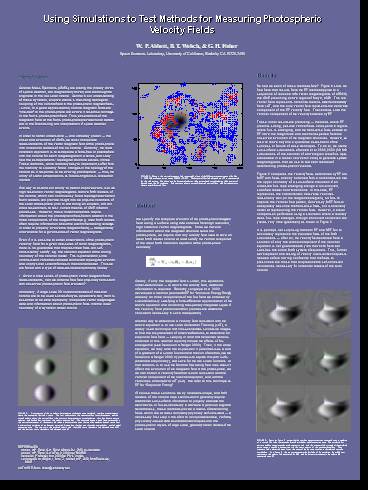
So how do each of these methods fare? Figure 1
shows the flow field that results from the EF
method applied to a sequence of reduced IVM
vector magnetograms of AR8210, the CME producing
active region of May 1, 1998. The red vector
field represents horizontal motions determined
directly from LCT, and the blue vector field
represents the transverse component of the EF
velocity field. The contours show the vertical
component of the velocity obtained by EF.
These initial results are promising --- the
areas where EF predicts strong, positive vertical
flows correspond to regions where flux is
emerging, and the transverse flows obtained via
EF have the magnitude and direction expected from
the observed evolution of the magnetic
structures. However, we wish to move beyond a
qualitative assessment of the success or failure
of these techniques. To do so, we use the
sub-surface simulations of Abbett et al. 2000,
2003 (3D MHD simulations of the evolution of
active region scale flux ropes embedded in a
model convection zone) to generate synthetic
magnetograms that we use to test each method of
determining photospheric velocities. Figure 2
compares the velocity fields determined by EF and
MEF with flows directly obtained from a
horizontal slice near the upper boundary of a
sub-surface simulation of an untwisted flux rope
emerging through a non-turbulent, stratified
model convection zone. In this case, EF
reproduces the characteristic transverse
velocities reasonably well (in the magnetized
region), but fails to capture the vertical flow
pattern Conversely, MEF fails to adequately
describe the transverse flows, but is nominally
better at reproducing the vertical flows.
However, a similar comparison performed using a
simulation where a relatively weak flux rope
emerges through a turbulent convection zone
yields very little agreement, as shown in Figure
3. It is perhaps not surprising that both EF and
MEF fail to accurately reproduce the simulated
flows of the MHD simulations --- after all, the
velocity field obtained from a solution of only
the vertical component of the induction equation
is not guaranteed to yield the vector field that
satisfies the entire MHD system of equations.
Thus, further development and testing of velocity
inversion techniques is needed before having
confidence that the flows so prescribed are those
that will produce the self-consistent boundaries
necessary for numerical models of the solar
corona.
- Coronal Mass Ejections (CMEs) are among the
primary drivers of space weather, are
magnetically driven, and are thought to originate
in the low solar corona. Central to our
understanding of these dynamic, eruptive events
is the strong topological coupling of the coronal
field to the photospheric magnetic field ---
since, to a good approximation, coronal magnetic
fields are line-tied to the photosphere and
evolve in response to changes in the Suns
photospheric field. Thus, observations of the
magnetic field at the Suns photosphere provide
crucial data to aid in the forecasting and
interpretation of space weather events. - In order to better understand --- and ultimately
predict --- the onset and evolution of CMEs, we
must incorporate measurements of the vector
magnetic field at the photosphere into numerical
models of the low corona. Currently, the most
common approach is to extrapolate a force-free or
potential field into the corona for each
magnetogram in a series, and study how the
extrapolations topological structure evolves in
time. These methods, while relatively easy to
implement, suffer from the inability to smoothly
follow changes in the topology of the corona as
it responds to the evolving photosphere ---
thus, the utility of static extrapolations as
forecasting tools is somewhat limited. - One way to extend our ability to predict eruptive
events is to use high resolution vector
magnetograms to drive MHD models of the corona,
which can continuously follow topological
evolution. Such models will provide insight into
the physical conditions of the solar atmosphere
prior to and during an eruption, and will allow
researchers to test current theories of CME
initiation processes. However, these numerical
models require information about the photospheric
flow-field in addition to the three components of
the magnetic field (e.g. ideal MHD models often
require information about the electric field
along cell edges in order to properly evolve the
magnetic field) --- data generally unavailable
for a given series of vector magnetograms. - Even if it is possible to obtain observations of
the photospheric velocity field for a given
time-series of vector magnetograms, there is no
guarantee that the prescribed flows will
self-consistently satisfy e.g. the induction
equation at the driving boundary of the coronal
model. This is problematic, since inconsistent
velocities can lead to incorrect topological
evolution and unphysical Lorentz forces in the
coronal model. Thus we are faced with a type of
data-assimilation problem, namely - Given a time series of photospheric vector
magnetic field measurements, can we obtain a
flow field physically consistent with observed
photospheric field evolution? - Ultimately, if large scale 3D numerical models of
the solar corona are to be used successfully as a
predictive tool, then it is essential to be able
to properly incorporate vector magnetogram data
and information about photospheric flows into the
lower boundary of a dynamic model corona.
FIGURE 1 AR8210 baby.
FIGURE 1 Shown is the vertical magnetic field
(grayscale) of one of the IVM vector magnetograms
of the May 1, 1998 CME producing active region
AR8210 (1940). The horizontal flow field
obtained via LCT is represented by the red
arrows. Also shown are the horizontal velocities
(blue arrows) and vertical velocities (blue
contours) derived using the EF technique. Solid
contours indicate outward-directed vertical
flows, while dotted contours indicate
inward-directed flows.
Method
We specify the temporal evolution of the
photospheric magnetic field along a surface using
data obtained from high resolution, high cadence
vector magnetograms. Since we have no
information about the magnetic structure below
the photosphere, we require that any velocity
field used to drive an ideal MHD model corona at
least satisfy the vertical component of the ideal
MHD induction equation at the photospheric
boundary
Clearly, if only the magnetic field is known,
this equation is under-determined --- to derive
the velocity field, additional information is
required. Recently, Longcope et al. 2002
developed a method (dubbed MEF for Minimum
Energy Fitting) whereby all three components of
the flow field are obtained by simultaneously
satisfying a finite-difference approximation of
the above equation and minimizing the spatially
integrated square of the velocity field (the
minimization provides the additional constraint
necessary to solve the equation). Another way to
determine a velocity field consistent with the
above equation is to use Local Correlation
Tracking (LCT), a widely used technique that
cross-correlates successive images to find the
displacement of observed features, to determine
an empirical flow field --- keeping in mind that
horizontal motions obtained in this manner
implicitly include the effects of flux emergence
(see Demoulin Berger 2003). Then, in the
above equation, we may write the expression in
parenthesis as a sum of a gradient of a scalar
function and the curl of another, use the
Demoulin Berger 2003 hypothesis to equate this
with uLCTBz (obtained empirically), and solve for
the two scalar functions. All that remains is to
use the fact that flow along field lines doesnt
affect the evolution of the magnetic field at the
photosphere, and we can obtain a velocity field
that is both consistent with the vertical
component of the induction equation, and with the
velocities obtained via LCT (uLCT). We refer to
this technique as EF for Empirical Fitting. Of
course these solutions are by no means unique,
and MHD models of the corona have stencils which
generally require additional sub-surface
information to properly evaluate the derivatives
or fluxes necessary to advance a particular
algorithm. Nonetheless, these methods provide a
means of determining flows which are at least
minimally physically self-consistent --- a
necessary first step in the effort to incorporate
reliable, verifiable, physically-based data
assimilation techniques into the photospheric
layers of large scale, global dynamic models of
the solar corona.
FIGURE 2 A comparison of the two velocity
determination techniques using simulated,
synthetic magnetograms where the associated flow
field is known. The first column shows the
transverse flows for all three cases, and the
second column shows the vertical flows (thin
contours denote negative vertical velocities,
thick lines denote positive velocities, and
dashed lines represent the velocity inversion
line). The grayscale image in each frame
corresponds to the vertical component of the
magnetic field (along a horizontal slice near the
top of the simulation domain) taken from a
sub-surface simulation of an buoyant, untwisted
Omega loop that has risen through a
non-turbulent, stratified model convection zone.
The top row is the simulated velocity field, the
middle row is the velocity field obtained using
MEF, and the bottom row is the velocity field
obtained using EF.
FIGURE 3 Same as Figure 2, except that the
synthetic magnetogram was generated using a
simulation of a twisted flux tube that ascends
through a turbulent model convection zone. The
simulated flow pattern includes super-granular
scale convective cells, and the magnetic field
strength of the simulated active region is
roughly in equipartition with the kinetic energy
of the strongest downflows. Thus, magnetic field
is advected away from the center of the flux
rope, resulting in the relatively complex
morphology. As in Figure 2, the top row
represents the flow fields of the simulation, the
middle row represents the velocity field
generated by MEF, and the bottom row represents
the velocity field generated using EF.
REFERENCES Abbett, W.P., Fisher, G.H., Fan
Y., Bercik D.J., 2003, ApJ submitted.
Abbett, W.P., Fisher, G.H. Fan, Y., 2000, ApJ,
540, 548. Demoulin, P. Berger, M.A., 2003,
Sol. Phys., in press. Longcope, D.W., Klapper,
I., Mikic, Z., Abbett, W.P., 2002, SHINE
workshop, Banff. AUTHOR E-MAIL
abbett_at_ssl.berkeley.edu
Recommended
