Linear filtering

1
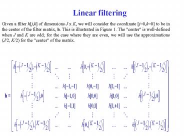
Linear filtering
Given a filter hj,k of dimensions J x K, we
will consider the coordinate j0,k0 to be in
the center of the filter matrix, h. This is
illustrated in Figure 1. The "center" is
well-defined when J and K are odd for the case
where they are even, we will use the
approximations (J/2, K/2) for the "center" of the
matrix.
2
Linear filtering
- frequencies in an image - spatial changes of
gray level or color - low frequencies - gradual
changes in gray level - high frequencies -
abrupt changes in gray level
3
In signal processing, the frequency of a signal
(audio signal) is a measure of the rate at which
the signal changes with time. Spatial frequency
is a measure of how rapidly brightness or color
varies as we traverse an image. Images in which
gray level varies slowly and smoothly are
characterized solely by components with low
spatial frequency. An image that is said to have
a "low frequency" if the change in intensity from
one pixel to the next is small. An image has
high frequency if the change in intensity
between adjacent pixels is large. High frequency
images tend to have a lot of detail and sharp
edges. Low frequency image tend to be soft or
fuzzy with little fine detail. . Note that
spatial frequencies occur within an image at any
given angle, not just along the horizontal or
vertical axes.
4
Low pass filtering
A low pass filter allows low spatial frequencies
to pass unchanged , but suppress high
frequencies. The low lass filet smoothes or blurs
the image. This tends to reduce noise, but also
obscures fine detail. The following shows a 3 x 3
kernel for performing a low-pass filter
operation. This is a simple kernel, each element
in the kernel has a value of 1. All pixels in the
input neighborhood will contribute an equal
amount of their intensity to the convoluted
output pixel. In other words, the output pixel is
just the simple average of the input neighborhood
pixels.
5
Mean filter is uniform kernel
The idea of mean filtering is simply to replace
each pixel value in an image with the mean
(average') value of its neighbors, including
itself. This has the effect of eliminating pixel
values which are unrepresentative of their
surroundings. Mean filtering is usually thought
of as a convolution filter. Like other
convolutions it is based around a kernel, which
represents the shape and size of the neighborhood
to be sampled when calculating the mean. Often a
33 square kernel is used, as shown in Figure 1,
although larger kernels (e.g. 55 squares) can be
used for more severe smoothing. (Note that a
small kernel can be applied more than once in
order to produce a similar but not identical
effect as a single pass with a large kernel.)
Any convolution kernel whose coefficients are all
positive will act as a low pass filter.
Coefficients sum to 1
6
Low pass filtering
The following example image illustrates the
frequency response of this filter, indicating
that low frequencies are permitted to pass
through unchanged but high frequencies are
rejected.
. Applying a low-pass filter also has the effect
of eliminating noise from an image, such as film
grain in a scanned image, since noise is nothing
more than very localized high frequencies.
Unfortunately, using this method to eliminate
grain also causes loss of sharp edge definition,
which is usually unacceptable.
7
Gaussian Smoothing Filters
The Gaussian smoothing operator is a 2-D
convolution operator that is used to blur'
images and remove detail and noise. In this
sense it is similar to the mean filter, but it
uses a different kernel that represents the shape
of a Gaussian (bell-shaped') hump. This kernel
has some special properties which are detailed
below. When we designing Gaussion linear
smoothing filters, the filter weights should be
chosen so that the filter has a single peak, call
the main lobe, and symmetry in the vertical and
horizontal directions. A typical pattern of
weights for a 3x3 smoothing filter is
The coefficients are samples from a
two-dimensional Gaussian function
8
How Gaussian Filter Works
The Gaussian distribution in 1-D has the form
where is the standard deviation of the
distribution. We have also assumed that the
distribution has a mean of zero (i.e. it is
centered on the line x0). The distribution is
illustrated in Figure 1.
Figure 1 1-D Gaussian distribution with mean 0
and 1
9
How Gaussian Filter Works
In 2-D, an isotropic (i.e. circularly symmetric)
Gaussian has the form
Figure 2 2-D Gaussian distribution with mean
(0,0) and ? 1
The idea of Gaussian smoothing is to use this 2-D
distribution as a point-spread' function, and
this is achieved by convolution. Since the image
is stored as a collection of discrete pixels we
need to produce a discrete approximation to the
Gaussian function before we can perform the
convolution.
10
Discrete approximation to the Gaussian function
In theory, the Gaussian distribution is non-zero
everywhere, which would require an infinitely
large convolution kernel, but in practice it is
effectively zero more than about three standard
deviations from the mean, and so we can truncate
the kernel at this point. Figure 3 shows a
suitable integer-valued convolution kernel that
approximates a Gaussian with ? of 1.0.
Figure 3 Discrete approximation to Gaussian
function with ? 1.0
11
Discrete approximation to the Gaussian function
Once a suitable kernel has been calculated, then
the Gaussian smoothing can be performed using
standard convolution methods. The convolution can
in fact be performed fairly quickly since the
equation for the 2-D isotropic Gaussian shown
above is separable into x and y components. Thus
the 2-D convolution can be performed by first
convolving with a 1-D Gaussian in the x
direction, and then convolving with another 1-D
Gaussian in the y direction. (The Gaussian is in
fact the only completely circularly symmetric
operator which can be decomposed in such a way.)
Figure 4 shows the 1-D x component kernel that
would be used to produce the full kernel shown in
Figure 3 (after scaling by 273 and rounding). The
y component is exactly the same but is oriented
vertically.
Figure 4 One of the pair of 1-D convolution
kernels used to calculate the full kernel shown
in Figure 3 more quickly.
12
Compute a Gaussian smoothing filter
A further way to compute a Gaussian smoothing
with a large standard deviation is to convolve an
image several times with a smaller Gaussian.
While this is computationally complex, it can
have applicability if the processing is carried
out using a hardware pipeline. The Gaussian
filter not only has utility in engineering
applications. It is also attracting attention
from computational biologists because it has been
attributed with some amount of biological
plausibility, e.g. some cells in the visual
pathways of the brain often have an approximately
Gaussian response.
13
Designing Gaussian filter
One approach to designing Gaussian filter is to
compute the mask weights directly from the
discrete Gaussian distribution
(1)
Where k is normalizing constant.
Choosing the value for ?2, we can evaluate (k)
over an n x n window to obtain a kernel, for
which the at 0,0 position equals 1. For
example choosing ?22 and n7 , from equation(1)
we will receive the array Kernel1.   To receive
integer values for the weights, we take the value
at one of the corners in the array, and choose k
such that this value becomes 1 .
14
Designing Gaussian filter
Kernel 1
15
Designing Gaussian filter
Using the above example, we get
Now , by multiplying , the rest of the weights by
k , we obtain Kernel 2
16
Kernel 2
17
Designing Gaussian filter
However , the weights , of the mask do not sum
to 1 . Therefore, when we performing the
convolution, the output pixel values must be
normalized by the sum of the mask weights to
ensure that regions of uniform intensity are not
affected. From the above example
Therefore the output image is
18
There are several advantages to using a Gaussian
filter
1 . Two dimensional , Gaussian function is
rotational symmetric. The kernel is rotationally
symmetric. This means that the amount of
smoothing performed by the filter will be the
same in all directions. 2.Large Gaussian filters
can be implemented very efficiently because
Causian functions are separable. Two-dimensional
Gausian convolution can be performed by
convolving the image with a one-dimensional
Caussian and then convolving the result with the
same one-dimensional filter oriented orthogonal
to the Gaussian used in the first stage.
19
Guidelines for Gaussian Filter Use
The effect of Gaussian smoothing is to blur an
image, in a similar fashion to the mean filter.
The degree of smoothing is determined by the
standard deviation of the Gaussian. (Larger
standard deviation Gaussians, of course, require
larger convolution kernels in order to be
accurately represented.) The Gaussian outputs a
weighted average' of each pixel's neighborhood,
with the average weighted more towards the value
of the central pixels. This is in contrast to the
mean filter's uniformly weighted average. Because
of this, a Gaussian provides gentler smoothing
and preserves edges better than a similarly sized
mean filter.
20
Guidelines for Gaussian Filter Use
We use input image

This image shows the effect of filtering with a
Gaussian of 1.0 (and kernel size 55).
Image 2 shows the effect of filtering with a
Gaussian of 4.0 (and kernel size 1515).
21
Gaussian Filter - Applications
Noise Reduction
Salt and pepper noise is challenging for a
Gaussian filter.
Image1 has been corrupted by 1 salt and pepper
noise (i.e. individual bits have been flipped
with probability 1).
Image 2 shows the result of Gaussian smoothing
(using the same convolution as above).
22
Gaussian Filter Noise Reduction
Increasing the standard deviation continues to
reduce/blur the intensity of the noise, but also
attenuates high frequency detail (e.g. edges)
significantly, as shown in this figure .
23
Low-pass filtering - Conclusions
- removes high frequencies - smooths or blurs
image - given by positive convolution
coefficients - coefficients sum to 1 - reduces
noise, but also removes meaningful information
from image - larger kernels remove more
noise, blur more, more costly to perform
convolution
24
High pass filtering
The classis 3 x 3 implementation is
The sum of the coefficients in this kernel is
zero. This means that, when the kernel is over an
area of constant or slowly varying grey level ,
the result of convolution is zero or some very
small number. However, when gray level is varying
rapidly within the neighborhood the result of
convolution can be a large number. The number can
be positive or negative and we need to choose an
output image presentation that supports negative
numbers.
25
High pass filtering
The high frequencies, or edges, of the image are
highlighted, while the low frequencies are
diminished. The visual impact of this is to make
the image appear sharpened.
High-Pass Filter Response Curve
26
High pass filtering
In high pass filtering the objective is to get
rid of the low frequency or slowly changing areas
of the image and to bring out the high frequency
or fast changing details in the image. This means
that if we were to high pass filter the box image
we would only see and outline of the box. The
edge of the box is the only place where the
neighboring pixels are different from one
another. There are many varied ways of
implementing a high pass filter. The simplest way
is to take a pixel and subtract it from its
neighbors. In this way we stress the difference
of the pixel from its neighbors. If the pixel is
in an area of little change, such as the middle
of the box, then the difference between the pixel
and its neighbors will be zero. However if the
pixel is on an edge of the box then the
difference will be large.
27
High pass filtering - Conclusions
- removes low frequencies - kernel has
positive coefficients at the center, negative
coefficients at the periphery - kernel
coefficients sum to zero - output will be
zero where gray level is constant, large positive
or negative where gray level is changing rapidly
28
High frequency emphasis
- compute weighted sum of original image and
results of high pas filter - use a kernal
similar to that of a high pass filter, but with
central coefficient greater than sum of periphery
coefficients.
29
What are the types of noise present in an image?
Images contain noise-pixels that arent what
they are supposed to be. The noise is nothing
more than very localized high frequencies. There
are various types of noise. They fall into two
major classes additive and multiplicative noise.
Additive noise is often assumed to be impulse
noise and Gaussian noise . Impulse noise
isolated bad pixels .In a binary image this means
that some black pixels become white and some
white pixels become black. This noise is called
salt and pepper noise . Additivesmall random
increment ( or -) at each pixel value. Additive
zero-mean Gaussian noise means that a value draw
from a zero-mean Gaussian probability density
function is added to the true value of every
pixel.. Multiplicative noise small random
increment at each pixel value. An example of
multiplicative noise is variable illumination.
30
Image independent noise
Image independent noise can often be described by
an additive noise model, where the recorded image
f(i,j) is the sum of the true image s(i,j) and
the noise n(i,j)
The noise n(i,j) is often zero-mean and described
by its variance ?n2 . The impact of the noise
on the image is often described by the signal to
noise ratio (SNR), which is given by
where ?s2 and ?f2 are the variances of the true
image and the recorded image, respectively.
31
Gaussian Noise

32
Noise which is dependent on the image data
In the second case of data-dependent noise (e.g.
arising when monochromatic radiation is scattered
from a surface whose roughness is of the order of
a wavelength, causing wave interference which
results in image speckle), it is possible to
model noise with a multiplicative, or non-linear,
model.
33
Salt and Pepper Noise
5 of the pixels (whose locations are chosen at
random) are set to the maximum value, producing
the snowy appearance.
Pixels have been set to 0 or 255 with probability
p1