
Minimal toy topology PowerPoint PPT Presentation
1 / 62
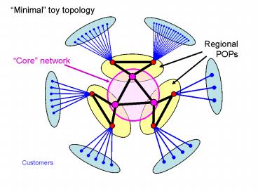
Title: Minimal toy topology
1
Minimal toy topology
Regional POPs
Core network
Customers
2
- Simplifying assumptions
- Physical and IP connectivity are identical (No
level 2 or MPLS) - Minimal geometry ( topology plus link speeds
and locations) - Aim to capture essence of topology
- Add complexity back in later
Line thickness roughly represents link bandwidth.
3
(No Transcript)
4
Minimal toy topology
Regional POPs
Core network
Customers
5
Router bandwidth is constrained.
Technically infeasible
Technically feasible
6
Customers with a variety of local connectivity
speeds.
high connectivity
Gateway routers
7
high connectivity
high speed
8
high speed
Technically infeasible
high connectivity
high speed
high connectivity
9
1
2
9
3
6
9
9
4
5
10
1
10
1
10
Total of nodes 56
1
2
56
9
3
6
9
9
4
5
10
1
10
1
11
Connectivity at edges?
1
2
56
9
3
6
9
9
?
?
4
5
10
Note Assume some unspecified local connectivity.
1
10
1
12
We are interested in distributions of core and
gateways so will largely ignore local
connectivity for now
Local
56
Core
?
?
10
9
6
5
4
log(rank)
3
2
Gateways
1
1
10
1
13
Scaling (Mandelbrot) or Power law
56
Do real networks have power law
connectivity? (There are people here better
qualified to answer than me, but very roughly
yes. And power laws per se are not important,
but heavy tails are.)
10
1
10
1
14
How do we define a simple, computable, yet
reasonable performance measure for such networks?
Proposal we define desired flows between
customers, which are then to be implemented by
flows in the network. We then can measure the
efficiency and perhaps robustness of the network
in producing these flows.
Well come back to this after a qualitative
discussion.
15
Varied customer demand
Conjecture
? Power law connectivity
56
10
Bandwidth constraints
1
10
1
16
Varied customer demand
What is the null hypothesis?
Interpret statistics as a probabilistic model.
? Power law connectivity
56
Eliminate design constraints.
10
Bandwidth constraints
1
10
1
17
Total of nodes 56
Total of links 72
Compute the degree distribution for random graph
with 56 nodes and 72 links. This has some
probability distribution (needs to be looked up).
Probability that there exists a node with degree
20 is vanishingly small.
18
Total of nodes 56
Therefore, vanishingly unlikely to have this
distribution in a purely random graph.
Total of links 72
1
10
0
Degree distribution for random graph with 56
nodes and 72 links????
10
-1
10
-2
10
Probability exists node with degree 20 is less
than ?1e-12????
-3
Can reject simplest null hypothesis.
10
-4
10
0
1
10
10
19
A more sophisticated null hypothesis.
? Power law connectivity
- Assume this scaling degree distribution but
otherwise random - Find typical or generic cases
- Standard statistical physics approach to complex
systems - Yields scale-free networks
56
10
1
10
1
20
What is the null hypothesis?
Interpret statistics as a probabilistic model.
? Power law connectivity
- Compare designed network with most likely
(maximum likelihood) random graph with same
connectivity degree
56
10
1
10
1
21
Null hypothesis
1
2
9
Total of links 72
Total of nodes 56
Total of links 72
10
1
22
Null hypothesis
1
2
9
Total of links 72
Most likely, highly connected nodes are connected
to each other.
10
1
23
- This is one of many possible definitions of
scale-free - Simply fill in links using the most probable
ones, in order, this will be the maximum
likelihood graph - Rearrange at random until it reaches statistical
steady state - others???
- All should give nearly the same thing, but the
max likelihood could be used as the canonical
scale-free network, and the likelihood (or some
related function) could serve as a measure of
nearness to scale-free.
24
- Note that there are two distinct notions here
- Max likelihood given a degree distribution (or
presumably any attributes, but were focusing on
degree distribution), identify the most likely
graph with that distribution among otherwise
random graphs - Scaling graphs with power law degree
distributions - Scale-free graphs are the max likelihood
scaling graphs. - Lets see what this looks like.
25
Redraw slightly and eliminate distinctions
between lines.
Reconnect edges to increase probability
This will quickly morph into a scale-free
graph. Completely random reconnections will get
there much more slowly.
26
Ignore the connections at the periphery for now.
Reconnect edges to increase probability
27
Reconnect edges to increase probability
28
Reconnect edges to increase probability
29
Reconnect edges to increase probability
30
Reconnect edges to increase probability
31
This is the scale-free network.
One problem is that it doesnt even connect to
all the nodes.
What to do at this point?
32
Recall that we had not specified additional local
connectivity. Could try to add that in, making
it try to get a fully connected graph.
Alternatively, we could just try to keep a power
law degree distribution and add links until it
becomes fully connected. Have to sort that out,
but will consider the qualitative features next.
33
Redrawn with core routers back in the middle.
34
Reconnect edges with same probability but
increase connectivity
And assume some local connections complete a
fully connected graph.
35
56
Note local connections not shown
These are extremely different, but have the same
connectivity distribution.
10
1
10
1
36
- Scale-rich
- Highly structured
- Self-dissimilar
- Efficient
- Robust
- Designed
- Scale-free
- Unstructured
- Self-similar
- Wasteful
- Fragile
- Emergent
37
- Scale-rich
- Each level has very different characteristics
- Pieces need not resemble the whole
- Scale-free
- Each level is similar
- Pieces resemble the whole
38
- Delete the highly connected node
- Only local loss
- Delete the highly connected node
- Global loss
- Remaining parts are still scale-free
39
- Delete the worst case node
- Relatively local loss
40
- The Internet does have huge fragilities
- Denial of service, DNS, BGP, etc
- The one fragility it doesnt have is deletion of
routers
41
- These are completely opposite extremes
- Scale-rich, Highly structured, Self-dissimilar,
Efficient, Robust, Designed - Vs. Scale-free, Unstructured, Self-similar,
Wasteful, Fragile, Emergent
42
- This is very different from the real Internet
- More importantly, it is very different from what
any Internet could possibly be
- Of course, no one would seriously propose that
the Internet really does look like this - Surely this is just a purely hypothetical null
hypothesis against which to compare more
sensible explanations. - Right?
- Scale-free
- Unstructured
- Self-similar
- Wasteful
- Fragile
- Emergent
43
- Typical of physics-based approaches to complex
networks - This approach dominates mainstream science
literature - Assume statistics describe an otherwise generic
configuration - Similar to edge-of-chaos, order for free,
criticality, order-disorder transitions,
emergence, - Essentially the same arguments and results hold
for biological networks
- Scale-free
- Unstructured
- Self-similar
- Wasteful
- Fragile
- Emergent
44
Scaling
56
10
Scale-free
1
10
1
Scale-rich
- Power laws (scaling) are consistent with either
scale-rich or scale-free - Scale-free is a natural and sophisticated null
hypothesis and is clearly refuted
45
Varied customer demand
Designed, Scale-rich, Highly structured,
Self-dissimilar, Efficient, Robust
56
? Power law connectivity
Bandwidth constraints
10
high speed
high connectivity
1
10
1
46
More realism
- Redundancy can easily give additional robustness
- Level 2 (ATM, Ethernet) and MPLS increase IP
versus physical connectivity - Real networks are obviously much more
complicated - Does this capture the essence of the degree
distribution? - What is a simple way to quantify efficiency and
robustness? - Could customer demand plus bandwidth constraints
give useful way to generate realistic
geometries ( topology plus locations plus
bandwidths)?
47
(No Transcript)
48
ASx
ASx
AS graph
ASy
ASy
49
- Every level is much more complicated.
50
Message Theory should help explain what is
observed and suggest what is necessary vs what is
accident.
56
10
Power laws
1
Scale-rich
10
1
high speed
Constraints
Scale-free
high connectivity
51
How do we define a simple, computable, yet
reasonable performance measure for such networks?
Proposal we define desired flows between
customers, which are then to be implemented by
flows in the network. We then can measure the
efficiency and perhaps robustness of the network
in producing these flows.
Well come back to this after a qualitative
discussion.
52
How do we define a simple, computable, yet
reasonable performance measure for such
networks? Below is a network with r5 routers and
n8 hosts in c3 clusters. There would be
n(n-1)/287/228 possible flows between all
hosts, which might get too big for larger
networks. So we can assume perhaps that there
will be 1337 local flows and then all
combinations of aggregated flows from the
clusters of local groups, which in this case
would be c(c-1)/23 flows.
53
For example.
3 aggregate flows
3 local flows
54
R has rows which correspond to nodes and columns
which correspond to links.
55
5
4
3
3
6
3
1
1
4
2
2
1
2
56
local flows
aggregate flows
matrix of flows on links
hosts
routers
5
4
3
3
6
3
1
1
4
2
representative set of flows
2
1
2
57
least squares (pseudo-inverse)
some norm?
absolute values
weighting matrix
5
4
3
3
6
3
1
1
4
2
2
1
2
58
- Could put link capacities into R perhaps, but
maybe want to use J to figure out what capacities
are needed and what the cost would be. - J as given here is a matrix with each column
giving the least squares link flows to realize
the desired traffic in the corresponding column
of X. - It might be better to solve linear programs with
constraints, but that will be more expensive, but
we should consider that. But something like this
should be ok.
59
- This has essentially the same features as
stoichiometry in biochemistry but is much
simpler, because - there is only one conserved quantity (flows or
packets) - the reactions are links, and thus all binary,
and thus representable as a graph
60
Stoichiometry
- We can define something similar for a biochemical
network, where R is the stoichiometry - The bigger problem is that we dont have an
obvious notion of scale-free here, since
reducing stoichiometry to a graph loses all
biological meaning - What we need to do is correctly characterize what
we mean here by - scaling
- max likelihood
61
- For both metabolism and the Internet graphs we
want to have a picture that looks something like
this. - Here bad performance means wasteful and fragile.
Empty
Scale-free
High
Likelihood
Possible, but to be avoided
optimal
Low
Good
Bad
Performance
62
- But also we want to make the point that this is a
very general picture, and applies to
edge-of-chaos, criticality, and self-organized
criticality as well.
Empty
EOC/SOC
High
Likelihood
optimal
Low
Good
Bad
Performance
Recommended
