Workshop Agenda

1
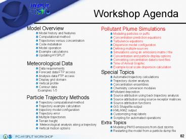
Workshop Agenda
82
82
2
Modeling Particle Motion or Particle
Distributions (Puffs)

• To compute air concentrations its necessary to
  follow all the particles needed to represent the
  pollutant distribution in space and time. This
  can be done explicitly by following the
  trajectory of each particle, where a random
  component is added to the mean velocity (from the
  meteorological model), to define the dispersion
  of the pollutant cloud. 
• In the horizontal, the computations can be
  represented by the following equations
• Xfinal(t ?t) Xmean(t ?t) U'(t
  ?t)?t, where, U'(t ?t) R(?t) U'(t) U''(1 -
  R(?t)2)0.5, (horiz. turbulent velocity)
• R(?t) exp(-?t/TLu), (auto-correlation
  coefficient)
• TLu is the Lagrangian time scale
• U'' su?, where ? is a random number with
  mean of 0 and s of 1. 
• The computations can be simplified, if instead of
  modeling the motion of each particle, we compute
  the trajectory of the mean particle position and
  the particle distribution. The standard deviation
  of the particle distribution can be computed from
  all the particles,
•        ______ s2  (Xi-Xm)2
• or it can be computed without following
  individual particles by assuming a distribution
  shape (puff) and relationship to the local
  turbulence.  Many different formulations can be
  found in the literature. dsh/dt v2 su su
  (Ku / TLu)0.5
• These computations are set in the Advanced /
  Configuration Setup / Concentration menu, which
  modifies the SETUP.CFG file.

83
3
Modeling Particle Motion or Particle
Distributions (Puffs)

• Below, note the initial differences between the
  simulation using the 3D particle distribution
  (left) and the top-hat puff center position
  method (right). Without the random motion
  component, the top-hat puff positions follow a
  straight line until vertical motions or
  horizontal divergence begins to act on the
  particles. In this particular case the primary
  reason for the expansion of the puff-particles is
  that they have mixed to near 500 meters where the
  winds are from the south-southwest and we are
  seeing the differential horizontal advection
  acting upon the particles.

3D Particle Distribution
Top-hat Puff Center Positions
84
4
Modeling Particle Motion or Particle
Distributions (Puffs)

• The previous example showed a snapshot of the
  particle or puff center positions after 6 hours. 
  Air concentrations are computed by summing each
  particles mass as it passes over the
  concentration grid.
• In the particle model mode, the concentration
  grid is treated as a matrix of cells, each with a
  volume defined by the grid dimensions. 
  Therefore, the concentration is just the particle
  mass divided by the cell volume
• 3D Particle      ?C q(?x ?y
  ?z)-1 Top-Hat           ?C q(? r2
  ?z)-1 Gaussian        ?C q(2? sh2 ?z)-1 e-
  0.5x2/sh2
• In the puff model mode, the concentration grid is
  considered as a matrix of sampling points, such
  that the puff only contributes to the
  concentration if it passes over the sampling
  point.  In the puff calculation mode it is
  possible for a puff to pass between points and
  not be shown on the display
• Top-Hat           ?C q(? r2
  ?zp)-1 Gaussian        ?C q(2? sh2 ?zp)-1 e-
  0.5x2/sh2

85
5
Modeling Particle Motion or Particle
Distributions (Puffs)

• Shown below are the concentration patterns
  associated with the particle (left) and puff
  (right) distributions from the previous example. 
  Note that the puff distribution is smoother but
  also initially somewhat broader.  In this
  particular case, the horizontal puff growth
  equations give larger values than the particle
  expansion. The noisy particle distribution
  indicates that more particles than 5000 used are
  needed to better represent the horizontal
  distribution.

3D Particle Distribution
Top-hat Puff Center Positions
86
6
Turbulence Equations
The method by which the meteorological data are
evaluated to determine the turbulent velocities,
used in either the puff or particle computation,
is set in the Advanced / Configuration Setup /
Concentration menu (below-left). Clicking on the
Configure the TURBULENCE method (7) button
produces the menu given below-right.
87
7
Turbulence Equations

• Turbulence Computation Methods
• Vertical Turbulence -  Determines how the
  turbulent velocity variances are computed from
  either the heat and momentum fluxes or the model
  profiles of wind and temperature. Two
  computational approaches (Beljaars/Holtslag and
  Kanthar/Clayson) are defined. Another option is
  the use the TKE (Turbulent Kinetic Energy)
  output from the meteorological model when
  available. In the default case the boundary layer
  velocity variances are defined as a function of
  u, w, and Zi.  For instance, in the
  stable/neutral boundary layer
• w'2 3.0 u2 (1 z/zi)3/2, u'2  4.0 u2
  (1 z/zi)3/2, v'2   4.5 u2 (1 z/zi)3/2
• If the TKE field is available from the
  meteorological model, then the velocity variances
  can be computed from its definition and the
  previous velocity variance equations to yield
  relationships with TKE
• E 0.5 (u2 v2 w2), w2 0.32 E,  u2
  0.74 E,  v2 0.85 E, u2   v2 0.36 w2
• Horizontal Turbulence - The default approach is
  to compute the horizontal mixing in proportion to
  the vertical mixing using one of the methods
  defined above. The original computation was to
  compute the mixing from the deformation of the
  horizontal wind field. In the event that
  horizontal variances are not computed, such as in
  the free troposphere, then the horizontal
  turbulence is assumed to equal the vertical
  turbulence
• u2 v2 w2

88
8
Turbulence Equations

• Turbulence Computation Methods (Cont.)
• Boundary layer stability Normally when
  turbulent fluxes (heat and momentum) are
  available from the meteorological data file, they
  are used to compute stability. Sometimes it may
  be desirable to force the stability to be
  computed from the wind and temperature profiles,
  especially if the fluxes represent long-time
  period averages rather than instantaneous values.
  If fluxes are not present, the profiles are used
  for the stability computation.
• Vertical Mixing Profile In previous versions
  the boundary layer mixing profile was replaced
  with its average value. This compensated for some
  meteorological data sets with poor vertical data
  resolution that might result in particles being
  trapped near the surface due to insufficient
  mixing. The current default is for no
  adjustments.
• Mixed Layer Depth Computation In addition as
  acting as a vertical lid to particle dispersion,
  the mixed layer depth is also used to scale the
  boundary layer mixing coefficients and computing
  turbulent fluxes from wind and temperature
  profiles. The default is to use the value
  provided by the meteorological model through the
  input data set. The computation defaults to
  compute the mixed layer depth from the
  temperature profile if the mixed layer or TKE
  fields are not available.

89
9
Turbulence Equations

• Turbulence Computation Methods (Cont.)
• Puff Growth Computation Method section is used to
  define either the default Linear or Square Root
  with time dispersion equation for the horizontal
  growth rate of puffs. This option does not affect
  particle dispersion. The linear with time
  approach suggests that not all turbulent scales
  have been sampled and square-root growth will be
  represented by the separation of puffs after
  splitting due to variations in the flow.
• Turbulence Aniosotropy Factors permits the user
  to set ratios of the vertical to the horizontal
  turbulence for daytime and nighttime. The ratio
  is defined as
• w2 /( u2 v2 )
• A zero value forces the model to compute a TKE
  ratio consistent with its turbulence
  parameterization. A non-zero value forces the
  vertical and horizontal values derived from the
  TKE to match the specified ratio.

10
Dispersion Model Configuration

• The control file (CONTROL) for dispersion
  simulations is configured from the Concentration
  / Setup Run menu tab.  The concentration setup
  layout is identical to the trajectory menu with
  the exception of an additional button to set the
  emissions, deposition, and concentration grid
  (top right).
• The Pollutant, Deposition and Grids setup button
  will bring up a submenu (lower right) with three
  options (Pollutant, Grids, Deposition).
• To make modifications, enter the number of
  pollutants to define in the Num box and then
  click on the Specie or Grid to access the
  next menu.
• The pollutant emission rate and deposition must
  be set for each pollutant. 
• Several independent concentration grids may be
  defined for each simulation. They may also be
  nested in space or time, if desired. 
  Concentrations for each pollutant species are
  output on all grids.

91
11
Dispersion Model Configuration

• Definition of Pollutant
• An arbitrary 4-character field identifies each
  pollutant.
• The Emission rate is defined in mass units per
  hour. The actual mass unit is not specified, so
  for instance, if the units are kg, then
  concentration output will be in kg/m3.  Any unit
  is acceptable, however some chemical conversion
  modules require specific units.
• The Hours of emission may be defined in
  fractional hours.
• The pollutant Release start can be set to any
  time at or after the start of the simulation.  As
  is true for all time units, zeros default to the
  simulation start time in the main menu.  Zero for
  the month and non-zero values for day and hour
  cause those values to be treated as relative to
  the simulation start time.

92
12
Dispersion Model Configuration

• Definition of Concentration Grid
• Each concentration grid must be defined. 
• Zeros for the grid center default to the source
  location. 
• The grid spacing is especially important in
  concentration computations in determining the
  cell size (particles) or sampling resolution
  (puffs). 
• When multiple levels are defined, each height
  represents the top of the cell (particles) or
  actual height (puffs). 
• The averaging time (Avg) starts at the sampling
  start time for the hours/minutes specified in the
  output interval. 
• Snapshot concentrations (Now) are defined as the
  average over one time-step at the time interval
  specified. Max will save the maximum
  concentration at each grid point over the
  duration of the output interval.

93
13
Example Dispersion Calculation

• Run the dispersion model using these settings
• Source St. Louis, MO, 38.75N, 90.37W _at_ 10.0 m
• Meteorology hysplit.t12z.ruc
• Emission 6 hrs beginning 1200 UTC on 17 Feb 2009
• Grid spacing 0.01 deg. lat/lon
• Grid span 20.0 deg. lat/lon
• 6 hour run time
• Output 6 hr average between the ground and 100
  m-agl
• Run Model (without SETUP)

94
14
Example Dispersion Calculation

• Results
• Change the map background file in the
  Concentration Display menu from arlmap to the
  map_county file that was distributed with the
  training meteorology.
• Set the contours to be UserSet and the interval
  1.0E-101.0E-121.0E-141.0E-16
• Set the zoom to 90 and then display the results.
• The resulting graphic should be the same as that
  shown (right). The noisy appearance indicates
  that not enough particles (2500 by default) were
  generated to adequately represent the dispersion
  at later times.

95
15
Example Dispersion Calculation

• Map Background Files
• The map_county file and other high resolution map
  backgrounds are ASCII files containing latitude
  and longitude locations of map boundaries. These
  files can be downloaded from the NOAA ARL website
  at http//www.arl.noaa.gov/ready/hysp_util.html
• Beginning with version 4.9, many of the
  Postscript based plotting programs have a new
  option to display map backgrounds from ESRI
  formatted shapefiles. Multiple shapefiles can be
  overlaid, each with its own color and line
  characteristics.
• This shapefile option is invoked by replacing the
  arlmap field with a file called shapefiles.txt.
  This file defines the characteristics of each map
  shapefile to be plotted.
• A sample shapefiles.txt file and a shapefile
  conversion of arlmap is given in the /shapefiles
  subdirectory. These files should be copied to
  the /working directory before they are to be
  used.
• The color and line parameters defined in
  shapefiles.txt will give a plot comparable to the
  default procedure using arlmap.
• More information can be found in the help
  document.

96
16
Example Dispersion Calculation

• All HYSPLIT simulations generate a text MESSAGE
  file, which contains diagnostic information about
  the calculation.  Use the View MESSAGES link from
  the Advanced menu tab to view the last MESSAGE
  file. In this case (below), at the end of the
  simulation, 5.9999892 units of mass were still
  on the domain. The vertical mass distribution
  showed more than 80 of the mass to be within 400
  m of the ground.  The vertical mass distribution
  is computed independently of the vertical
  concentration grid.

97
17
Defining Multiple Sources

• Now run the dispersion model for 2 sources
  using these settings
• Source1 38.75N, 90.37W _at_ 10.0 m
• Source 2 38.75N, 91.05W _at_ 10.0 m
• Meteorology hysplit.t12z.ruc
• 6 hour run time
• Emission 6 hrs beginning 1200 UTC on 17 Feb
  2009
• Output 6 hr average concentration between the
  ground and 100 m-agl
• Run Model

98
18
Defining Multiple Sources

• Set the zoom to 70 and display the results.
• A second source added at location 38.75N and
  91.50W results in two adjacent, similar plumes. 
• Note that the emission rate of 1 unit per hour
  over 6 hours is applied to each source
  individually and therefore the concentrations are
  similar to the last case.

99
19
Defining Multiple Sources

• The emission rate can be set for each source by
  including that information after the release
  height in the Starting Location Setup menu. (A
  fifth field can be added that sets an initial
  plume area in square-meters, but is only valid
  for puff simulations.)
• In the example shown here (top right), the
  emission rate of the second source has been
  increased to 10 units/hr
• To display the same concentration levels as the
  last graphic, make sure the UserSet is set to
  1.0E-101.0E-121.0E-141.0E-16
• The concentrations in the second plume (right)
  have increased by the same amount as the emission
  increase (10).

100
20
Simulation using anEmission Matrix

• Emission Matrix
• An emission matrix is defined using three
  locations the first two represent the lower left
  and upper right grid corners, respectively, and
  the third represents the grid spacing.
• Example to run (below)  Start sources every 1
  degree between the grid corners (38.0, -92.0) and
  (41.0, -89.0).
• Configure the model to run with 25,000 particles
  per emission cycle (option 4) and increase the
  maximum number of particles to at least 50,000 in
  the Advanced / Configuration Setup /
  Concentration menu.
• Leave all other parameters the same as the last
  St. Louis example, and run the model from the
  Concentration / Special Runs / Matrix menu option
  (Run using SETUP file).
• Click Continue when asked to run the matrix.
• Prior to running the model, the CONTROL file is
  redefined with 16 starting locations (right).

101
21
Simulation using an Emission Matrix

• The result (top right) shows 16 plumes over a
  uniform 1.0 degree grid.
• To make the graphic less noisy, from the
  Concentration Display menu, turn off the source
  location labeling and remove the black contour
  lines from the graphic by setting the contour
  outlines to none (see below).
• Execute the display to create a considerably
  simplified graphic (right, bottom).

102
22
Simulation using an Emissions File

• Emission File
• In this approach, an EMITIMES file is used to
  configure more complex point source emissions
  scenarios.
• In the standard model simulation, the CONTROL
  file can only be used to define one pollutant
  release cycle which applies equally to all source
  locations. Although multiple release cycles can
  be defined, they must all be at the same
  interval.
• With this update in the point source emissions
  file structure, multiple release locations can
  each have their own emission characteristics,
  each with different pollutants, if desired.
• Furthermore, multiple emission cycles, at
  non-regular intervals can also be defined. By
  appropriately locating multiple sources in space
  and time, line-source as well as other
  non-regular emissions configurations can be
  created.
• Information on the format of the emissions file
  and the emission text file can be found in the
  HYSPLIT User's Guide under Advanced /
  Configuration Setup / Emissions File (S417).

103
23
Simulation using an Emissions File

• To run the simulation with 3 sources, define 3
  sources as usual in the Concentration Setup menu.
  (The number of source locations defined in the
  Setup menu must match the number of sources in
  the EMITIMES setup, but the location of each is
  overridden by the EMITIMES file).
• From the Advanced / Configuration Setup /
  Emissions File menu enter the number of sources
  to define and click Configure Locations. In
  this case, 3.
• Next, click on the Location number to open a
  menu to define each source.
• For this example, we will define 3 sources with
  varying emission release rates and durations (all
  starting at 1200 UTC February 17, 2009)
• Source 1 38.0 -92.0 10 m, 6 hour emission, 1000
  units/hour
• Source 2 39.5 -90.5 10 m, 3 hour emission, 100
  unts/hour
• Source 3 41.0 -89.0 10 m, 1 hour emission, 1
  unit/hour
• Note, the GUI menu only supports the creation of
  a EMITIMES file for one pollutant for one
  emission cycle. If multiple pollutants are
  defined, or multiple cycles are required, then
  the file must be edited manually by duplicating
  the emission record at each location for all
  pollutants in the order they are defined in the
  CONTROL file.

104
24
Simulations using an Emissions File

• Next, the EMITIMES file must be defined in the
  namelist (SETUP.CFG) file. From the Advanced /
  Configuration Setup / Concentration, select
  Define EMISSION CYCLING or input file (6). Click
  on the Default Name button under Optional Point
  Source Emission File to set the emission file
  name to EMITTIMES. Click Save and Save again.
• Run the model using SETUP file (keep all other
  parameters the same as the previous Matrix
  approach calculation).
• The EMITIMES file (below) created in the \working
  directory contains information on the 3 sources
  just defined.

105
25
Simulations using an Emissions File

• Before displaying the results, turn off the Label
  Source since the 3 sources defined initially in
  Concentration Setup were not the same 3 sources
  we defined in the EMITIMES file, otherwise a star
  will be indicated at a non-source location. Also,
  to reduce the clutter, set the Contour drawing
  options to None and set the Zoom to 100.
• The result (right) shows 3 sources with the
  northern-most source having the lowest
  concentration and the southern-most source having
  the largest concentration, as expected.

106
26
Concentration and Particle Display Options
Now, we will look at the particle distributions
for the St. Louis case for various source terms.

• Setup the following run
• Delete the emission.txt and emission.asc files
  from the working directory if used previously.
• Source 38.75N, 91.37W _at_ 10.0 m
• Meteorology hysplit.t12z.ruc
• Emission 6 hrs beginning 1200 UTC on 17 Feb 2009
• Output snapshot at 6 hours between the ground
  and 100 m-agl
• 3-D particle horizontal and vertical
• 500 particles released per cycle
• Dump the particles to a file called PARDUMP after
  6 hours (menu option 9, right)
• Run Model (using SETUP)

107
27
Concentration and Particle Display Options

• Results
• Turn source labeling back on in the Concentration
  Display menu and execute the display.
• The resulting graphic should be the same as that
  shown (right).
• The concentration output clearly shows a noisy
  pattern indicating too few particles were defined
  to adequately represent the plume.

108
28
Concentration and Particle Display Options

• Setup the following runs
• Rerun the last case, but use 5,000 and 50,000
  particles.
• Make sure the maximum number of particles is
  greater than 50,000.
• Although this is a snapshot (not an average over
  time), the particles are beginning to better
  define the plume, but at the expense of longer
  computational time.

5,000 Particles
50,000 Particles
109
29
Concentration and Particle Display Options

• Results
• To speed up the run without loosing the plume
  structure, change the type of run from a 3D
  particle to a top-hat-horizontal
  particle-vertical and reduce the number of
  particles to 500.
• The resulting plume (right) covers most of the
  footprint as the 50,000 3D particle run.

110
30
Concentration and Particle Display Options

• Particle Display
• In addition to the standard display of particle
  concentrations, individual particle positions can
  also be displayed on a map.
• The Concentration / Display / Particle menu
  (right) has options to show snapshot particle
  distributions, assuming that the particle dump
  option was set in the Advanced / Configuration
  Setup / Concentration menu before running the
  particle simulation.
• Horizontal, vertical, and cross-sectional views
  are available.
• Other options include color-coding the particles
  by mass size (Mass Sizing), by height (Color
  Scale) or output as a shapefile (GIS).

31
Concentration and Particle Display Options

• Particle Display
• Rerun the 5,000 3D particle simulation and set
  the first output of particle dump to 6 hours to
  produce a PARDUMP binary particle dump file in
  the /working directory.
• Then, from the Particle Display menu, select the
  View Type to be Cross-section, check the Color
  Scale option, and set the Zoom to 80.
• As seen in the graphic (right), the center line
  of the vertical cross-section is drawn
  automatically based upon the particle
  distribution.
• The particles toward the northeast are at a
  higher level than those closer to the source.

32
Concentration and Particle Display Options

• Pointer Select Concentration Display
• Another display option is to view the
  concentration values directly on the grid without
  any interpolation through the Concentration /
  Display / Concentration / Pointer Select menu
  (upper right).
• This option will draw the entire concentration
  domain as defined in the concentration grid setup
  menu. The grid span would need to be reduced to
  zoom in on the area of interest.
• Click on the initial map domain image with the
  right mouse button to display the concentrations
  (right). In this case the full 20 x 20 degree
  concentration grid defined previously covers an
  area much larger than the plume.

33
Concentration and Particle Display Options

• Color Fill of the Concentration Grid
• A generic Postscript equivalent to the Pointer
  Select is the Grid Values display option. Grid
  values runs the gridplot program to view the
  concentration values directly on the grid without
  any interpolation.
• Gridplot was designed to plot global sized
  concentration grids, although any sized grid can
  be displayed.
• This option will draw the entire concentration
  domain as defined in the concentration grid setup
  menu and there are no zoom options. The grid
  span would need to be reduced to zoom in on the
  area of interest.
• Options are available to set the lowest
  concentration level and the contour interval.

34
Converting Concentration Data to Text Files

• The concentration output file is in a binary
  format, however there are several options
  available through the Concentration / Utilities
  menu that can be used to convert the
  concentration data to other formats.
• First, prepare a multi-time period output file by
  setting up a simulation as in the previous
  example, but with the following changes
• Top-hat-horizontal particle-vertical,
• No particle dump interval (0),
• 6 hour simulation,
• 1 hour release at 1200 UTC 17 Feb 2009,
• 500 particles, and
• 1 hour average concentrations.
• Check the Fix-Exp box in the Display menu to keep
  the contours constant and you may need to change
  the name of the output file from partplot to
  concplot.
• After displaying the Postscript output, create an
  animated gif image by using the Concentration /
  Utilities / Convert Postscript menu by checking
  the animate box in the Postscript Conversion
  menu.
• The plume moves north and decreases in
  concentration.

35
Converting Concentration Data to Text Files

• Time Series Data Extraction
• Next, select the Concentration / Utilities / Grid
  to Station menu (right).
• Select a point downwind in the plume (39.1N,
  91.4W),
• Give it a unique Integer ID (3991),
• Set the Concentration Multiplier to 1.0,
• and choose a Log Ordinate scale.
• Click Extract Data and an ASCII con2stn.txt file
  will be created in the /working directory with
  the concentration values interpolated to that
  location.  (An input file with the station
  locations must be created to do multiple
  locations).
• Selecting the Display Time Series Yes button
  results in the creation of a time series plot
  (right) in the /working directory called
  timeplot.ps. In this case the peak concentration
  occurred at 1300 UTC on 17 February 2009.

36
Converting Concentration Data to Text Files

• The Concentration / Utilities / Convert to ASCII
  menu will convert every non-zero grid point value
  to its ASCII equivalent, writing the output to
  one file per time period unless you specify
  Single File.
• Files are labeled according to the name of the
  binary file, Julian day, and hour of the sampling
  period.
• See the contents of this file for the output from
  the first time period (1300 UTC).
• This file can useful when importing the data into
  other mapping applications.
• The concentrations and depositions can be
  multiplied by a conversion factor with the
  Conversion Options.

37
Time of Arrival Graphic

• The Concentration / Display / Arrival menu will
  plot a map of the time of arrival of the plume.
• In this case, since we ran a 6 hour simulation,
  the Number of contours is set to 6 (hours).
  Leaving the Time difference as -1, indicates that
  the program will use the concentration averaging
  time as the default contour interval.
• A Threshold value can also be set.
• The resulting graphic show the location of the
  plume at hourly intervals indicated by blue to
  green shading.

38
Example Local Scale Dispersion Calculation

• HYSPLIT can be configured for applications such
  as emergency response, when the scale of the
  simulation is on the order of 1-30 km.
• For this example, set up the run as shown below
  for Washington, D.C.
• Click Reset from the main menu
• 38.880N 77.027W _at_10m and 100m,
• 1200 UTC 17 February 2009,
• NAM 12 km NE tile forecast data,
• 1-hr emission and simulation,
• 1-hr average concentration,
• Lat/lon Grid Resolution of 0.001 degrees, and
  Grid Span of 1.0 degrees lat/lon.
• Using the Advanced / Configuration Setup /
  Concentration menu, set
• 3-D particle horizontal and vertical method,
• 5000 particles released per cycle,
• 10000 maximum number of particles, and
• Run Model using SETUP file

39
Example Local Scale Dispersion Calculation

• After running the model, set the Concentration
  Display menu to the following (right)
• Output File concplot
• Number of rings to 4 every 10 km
• Map background to /working/map_county
• Zoom to 90
• Dyn-Exp contours
• Turn on the contour outlines (Color) 
• Turn on the Google Earth option

40
Example Local Scale Dispersion Calculation

• The resulting plume (below left) produces a
  narrow plume moving south-southeast into southern
  Maryland over the 1 hour period.
• As will be discussed later, the Google Earth file
  (HYSPLITconc.kmz) was created and allows the
  emergency manager to overlay the plume with other
  geographic features (below right). This file can
  be provided directly to the emergency manager.

41
Example Local Scale Dispersion Calculation

• Now assume the release was very small and only
  lasted 15 minutes. Use the Concentration setup /
  Pollutant, Deposition and Grids setup menu
  (right) to define a 15 minute (0.25h) release of
  one unit of mass. Note that since the release
  rate required is per hour, you will need to
  multiply the mass by 4 in this case.
• Also, change the averaging period to 10 minutes
  over the 1 hour simulation, which can be defined
  in the Concentration Grid Setup menu.
• Run the model and create an animated GIF (right).
  To keep the contours from changing as the
  concentrations decrease, you may want to fix the
  contours by checking Fix-Exp box in the
  Concentration Display menu and set the Contour
  drawing options to none.