BASIC BOND VALUATION MODEL

1
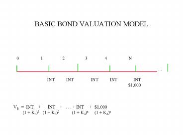
BASIC BOND VALUATION MODEL
0 1 2
3 4 N
. .
INT INT INT INT
INT
1,000
VB INT INT . . . INT
1,000 (1 Kd)1 (1 Kd)2
(1 Kd)n (1 Kd)n
2
THINGS THAT AFFECT BOND VALUE

• ANYTHING THAT AFFECTS (CHANGES) Kd
• E.G., CHANGING INFLATION EXPECTATIONS, CHANGES IN
  THE REAL RATE (K), CREDIT RISK, LIQUIDITY,
  MATURITY RISK.

3
BASIC BOND VALUATION MODEL
0 1 2
3 4 N
. .
INT INT INT INT
INT
1,000
VB INT INT . . . INT
1,000 (1 Kd)1 (1 Kd)2
(1 Kd)n (1 Kd)n
4
VB INT(PVIFA, N, Kd) 1,000(PVIF, N, Kd)
5
SIMPLE EXAMPLE ASSUMING ONE INTERESTPAYMENT PER
YEAR
PAR VALUE 1,000 (DOESNT CHANGE) COUPON RATE
12 (DOESNT CHANGE) INTEREST 1,000 X 12
120 (DOESNT CHANGE) YIELD (Kd) 12 (DOES
CHANGE) MATURITY 10 YEARS (DOES CHANGE) VB
INT(PVIFA, N, Kd) 1,000(PVIF, N, Kd)
120(PVIFA, 12, 12) 1,000(PVIF, 12, 12)
1,000
6
CALCULATOR PROCEDURE USING TVM BUTTONS

• SET P/Y 1
• ENTER 10 FOR N
• ENTER 120 FOR PMT
• ENTER 1,000 FOR FV
• ENTER 12 FOR I/Y
• CPT PV 1,000

7
VB PAR VALUE
WHEN Kd COUPON RATE
8
VB? NOT EQUAL PAR VALUE
WHEN Kd IS NOT EQUAL TO COUPON RATE.
9
AS Kd RISES

• BOND VALUES FALL
• VB INT INT . . . INT
  1,000
• (1 Kd)1 (1 Kd)2 (1 Kd)n
  (1 Kd)n

10
EXAMPLE WITH YIELD RISING
PAR VALUE 1,000 COUPON RATE 12 INTEREST
1,000 X 12 120 YIELD (Kd) 16 MATURITY
10 YEARS VB 120(PVIFA, 10, 16) 1,000
(PVIF, 10, 16) 806.67 (LESS THAN
1,000 SELLS AT A
DISCOUNT FROM PAR)
11
AS Kd FALLS

• BOND VALUES RISE
• VB INT INT . . . INT
  1,000
• (1 Kd)1 (1 Kd)2 (1 Kd)n
  (1 Kd)n

12
EXAMPLE WITH YIELD FALLING
PAR VALUE 1,000 COUPON RATE 12 INTEREST
1,000 X 12 120 YIELD (Kd) 8 MATURITY
10 YEARS
VB 120(PVIFA, 10, 8) 1,000(PVIF, 10, 8)
1,268.40 (MORE THAN 1,000 SELLS
AT A PREMIUM TO PAR)
13
A BONDS PRICE APPROACHES ITS PAR VALUE AS BOND
APPROACHES MATURITY
BOND PRICE
PATH OF PREMIUM BOND
1,000
PATH OF A DISCOUNT BOND
TIME
14
FINDING A BONDS YIELD (Kd), GIVENITS PRICE (VB)
PAR 1,000 COUPON RATE 8 PRICE 701.22 N
20 Kd ?
701.22 80 80 . .
. 1,080 (1 Kd)1 (1
Kd)2 (1 Kd)20
15
CALCULATOR APPROACH
701.22 80(PVIFA, 20, Kd) 1,000(PVIF, 20,
Kd)
-701.22 PV 80 PMT 20 N 1,000 FV CPT I/Y
12
16
INTEREST RATE RISK

• THE RISK THAT A BONDS PRICE WILL FALL BELOW ITS
  PAR VALUE BECAUSE OF A RISE IN INTEREST RATES.
• THE MORE DISTANT A BONDS MATURITY, THE GREATER
  ITS EXPOSURE TO INTEREST RATE RISK.

17
INTEREST RATE RISK EXAMPLE
PAR 1,000 COUPON RATE 10 (ANNUAL)
BOND VALUES Kd
2 YEAR BOND 20 YEAR BOND 6
1,073.34
1,458.80 8 1,035.67
1,196.36 12
966.20
850.61 14 934.13
735.07 16
903.67 644.27
18
FINDING BOND VALUES IN THE REALWORLD USING
SEMIANNUAL COMPOUNDING

• VB INT/2 INT/2 . . .
  INT/2 1,000
• (1 Kd/2)1 (1 Kd/2)2
  (1 Kd/2)nx2
• P/Y 2
• VB INT/2(PVIFA, 2N, Kd) 1,000(PVIF, 2N,
  Kd)

19
EXAMPLE OF BOND VALUATION WITHSEMIANNUAL
COMPOUNDING
PAR VALUE 1,000 COUPON RATE 8 Kd 12 N
20 VB 80/2(PVIFA, 2X20N, 12/2) 1,000(PVIF,
2X20N, 12/2) 699.07
20
FINDING BOND YIELDS WITH SEMIANNUALCOMPOUNDING

• VB INT/2 INT/2 . . .
  INT/2 1,000
• (1 Kd/2)1 (1 Kd/2)2
  (1 Kd/2)n

PAR VALUE 1,000 COUPON RATE 8 Kd ? N
20 VB 699.07
21
EXAMPLE FINDING BOND YIELDS WITH SEMIANNUAL
COMPOUNDING
699.07 80/2(PVIFA, 2X20N, Kd/2) 1,000(PVIF,
2X20N, Kd/2)
SDT 1.0196 CPN 8 RDT 1.0116 RV100 360 2/Y P
RI 69.907 YLD CPT 12
22
PREFERRED STOCK

• HAS ELEMENTS OF BOTH STOCK AND BONDS
• FIXED NON TAXDEDUCTIBLE DIVIDENDS
• CAN BE SKIPPED
• ALL PREFERRED DIVIDENDS IN ARREARS MUST BE PAID
  BEFORE COMMON STOCK DIVIDENDS PAID

23
PREFERRED STOCK
VALUED AS A CONSTANT STREAM OF PAYMENTS OR AS A
PERPETUITY PVPS DPS KPS IMPLIES
KPS DPS PVPS
24
PREFERRED STOCK EXAMPLE
KPS 12 DPS 8 PVBS 8/.12 66.67
25
COMMON STOCK

• DIVIDENDS BY COMPANY OPTIONAL
• DIVIDENDS CAN VARY
• VALUATION DEPENDS ON ASSUMPTION OF CONSTANT
  GROWTH OF DIVIDENDS

26
COMMON STOCK CASH FLOWS
0 1 2 3

• ?

. . . .
D0 D1 D2
D3
P0 D1 D2
D3 . . . (1 Ks)1 (1
Ks)2 (1 Ks)3
(NOT PRACTICAL)
27
TO PERMIT COMMON STOCK VALUATION,ONE OF TWO
ASSUMPTIONS MUST BE MADE

• DIVIDEND GROWTH IS ZERO (AS FOR PREFERRED STOCK)
  OR
• DIVIDEND GROWTH IS CONSTANT

28
CONSTANT GROWTH MODEL AKAGORDON GROWTH MODEL

• ASSUMES DIVIDENDS GROW AT A CONSTANT RATE
• VALUES DIVIDENDS AT THE START OF CONSTANT GROWTH
• THE START OF CONSTANT GROWTH CAN OCCUR ANY TIME

29
CONSTANT GROWTH EQUATION
P0 Dg(1 g) Ks - g Ks gt g
DEFINE TERMS
DISCUSS IMPLICATIONS
30
CONSTANT GROWTH EXAMPLE
D0 2 Ks 10 g 8 CONSTANT GROWTH
STARTS AT TIME ZERO P0 2(1 .08) 108
.10 - .08
31
CONSTANT GROWTH MODEL WITHSUPERNORMAL GROWTH
ASSUMES NONCONSTANT HIGH GROWTH IN EARLIER YEARS,
THEN CONSTANT GROWTH THEREAFTER
0 1 2
3
4
g1
g2
g3
g3
g3
. . .
32
EXAMPLE SUPERNORMAL GROWTH

• YOU ARE CONSIDERING THE PURCHASE OF AN IPO CALLED
  COMPUTER SOFT, INC.
• EARNINGS AND DIVIDENDS EXPECTED TO GROW AT 20
  DURING YEAR 1, 15 DURING YEAR 2, AND 12
  THEREAFTER.
• D0 1.50 Ks 15

33
SUPERNORMAL GROWTH EXAMPLE
0 1 2
3
20
15
12
12
1.50
1.80
2.07
2.32
1.50(1.2)
1.8(1.15)
2.07(1.12)
1.80 2.07
2.32/(.15 - .12) P0 (1.15)1
(1.15)2 (1.15)2
61.61
34
A BRIEF LECTURE ON THE TERM STRUCTURE OF INTEREST
RATES
Term structure a schedule showing the yields on
securities alike in
all respects except their term to
maturity.
Example
U.S. Treasury Bonds
Years to maturity Yield 1
5 2
5.5 3
6
35
Yield Curve
The graph of the term structure is called the
yield curve
.
Yield
.
6 5.5 5
.
years
1 2 3
36
Shape of the Yield Curve
The yield curve can be positively sloped, flat or
negatively Sloped. Positive implies
short-term rates are expected to rise Flat
suggests no change in short-term rates Negative
short-term rates are expected to fall
37
Theories explaining the shape of the yield curve

• Expectations Hypothesis
• Market Segmentations Hypothesis
• Liquidity Preference Hypothesis

38
Expectations Hypothesis
Says spot rates are the average of expected
future Short-term rates. A spot rate is a rate
observable on a security today Example of spot
rates Yield on a one year bond 5
Yield on a two year
bond 5.5
Yield on a three year bond 6
39
Rationale behind the Expectations Theory
The Expectations theory is based on the notion
that when Investing over a period greater than
one year, investors Have a choice of investing in
a long-term bond or a series Of one year bonds.
For investors to be indifferent between This
choice, long-term rates have to be equal to the
average Of the expected future short-term rates
on the one year bonds.
40
Mathematical Rationale
(1 rn)n (1 r1)(1 r2)(1 r3) . . .(1
fn)
41
Alternatively . . .
(1 rn)n (1 rn-1)n-1(1 fn) This
implies (1 rn)n fn
-1 Using this
equation (1 rn-1)n-1
we can solve for the
forward rate
42
Example
0 1 2 3 4
10
12
The yield on a 4 year Treasury bond is 12 The
yield on a 3 year Treasury bond is 10 Find the
expected one-year rate during year 4 f4
(1.12)4 -1 1.5735 -1
18.22 (1.10)3
1.3310
43
Market Segmentations Hypothesis
The theory that investors and borrowers have
preferred maturity Habitats. The yield curve is
thought to be determined by the Demand-supply
relationship within each habitat
44
Liquidity Preference Hypothesis
Assumes the yield curve is upward sloping
(usually) because Investors would rather lend
short-term and borrowers would Rather borrow
long-term