
Contaminant transport in the subsurface PowerPoint PPT Presentation
1 / 31
Title: Contaminant transport in the subsurface
1
(No Transcript)
2
(No Transcript)
3
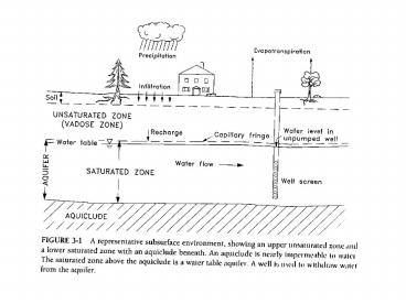
Contaminant transport in the subsurface
- Two phase medium VOIDS SOLIDS
- The voids typically filled with some fluid
liquid or gas, sometimes both, thus giving a
three phase medium
4
Darcys law
h L K L/T
5
Constant Head Apparatus (in lab)
6
(No Transcript)
7
Continuity equation, incompressible fluid
Dimensions 1/T, multiplying by density gives
M/L3T
Dimensions 1/L
8
(No Transcript)
9
Velocities in two phase media
10
(No Transcript)
11
- Fig 6.2 BR
12
Dispersive flux in the subsurface
- For a one dimensional flow characterized by a
uniform seepage velocity vx, we might expect the
dispersion coefficients D to be proportional to
velocity - Dispersivity is a characteristic of the system
that will need to be determined experimentally
(recall determination of dispersion coefficients
in the atmosphere and surface waters)
13
Diffusive and dispersive fluxes in the subsurface
- Since the diffusive and dispersive fluxes are
defined similarly, if we let Dx represent the sum
of diffusivity and dispersion coefficient both
fluxes will have been included in the
advection-diffusion equation. Thus - We have independent means for measuring
diffusivity (Dd ) which, is determined by
temperature, pressure, and molecular properties
of the diffusing molecule as well as the mixture
in which it is diffusing - (recall the theoretical, empirical correlations
for gases and liquids)
14
Tortuosity
- The tortuous path taken in the x direction by
diffusing molecules means that the diffusive flux
is less than the flux in the case of an available
straight path. - We can define tortuosity as
- see (Fig 6.2 BRN)
- Then our dispersion coefficient expression
becomes - t lt 1, 0.56 0.8 for granular media (Bear,
1972) - Not easy to measure independently
15
Adsorption
- The adhesion of a component in the fluid to the
solid surface. - Depends on
- Temperature
- Solute
- Solid
- C mass of solute per volume of fluid
- S mass of solute per mass of dry solid
16
S
17
(No Transcript)
18
Accumulation in two phases
19
(No Transcript)
20
- Figure 6.1 BR
21
Advection-dispersion in two phases(no decay)
22
- Recall the case examined before
- With initial and boundary conditions
- S(0,t) So for all tgt0
- ?S/?x 0 at xL
- S(x,0) 0 at t0
- And analytical solution
23
- In BR notation for subsurface contaminant
transport, assuming constant Dx - Initial and boundary conditions
- C(0,t) Co for all tgt0
- ?C/?x 0, at xL
- C(x,0) 0 at t0
- Analytical solution (Eqn 6.17 BR) at xL
24
- The previous formulation describes a tracer (dye)
test (step input) in a column of porous material. - The amount of liquid passed through the column is
usually measured in number U of pore volumes (Eqn
6.39 BR) - When the solution is expressed in terms of U and
plotted on appropriate coordinates, the
dispersion coefficient can be obtained from the
slope. (See Fig 6.10a BR)
25
- Figure 6.10a
26
Dispersion in a sand column, Example 6.4
BRN(see Ex6_4BR.xls)
27
PARTICLE SIZE DISTRIBUTION
- Gaussian, or normal
28
ALTERNATE FORM FOR GAUSSIAN DISTRIBUTION
29
GAUSSIAN DISTRIBUTION, INTEGRATED FORM
- (Table 8.3 de Nevers)
- Probability scale a scale linear in z
- Gaussian distribution gives linear plot on
- normal (y axis) vs probability (x axis)
coordinates - Slope standard deviation
- mean value is at z 0
30
Table 8.3 de Nevers
- Values of the cumulative frequency integral
31
Figure 8.8 de Nevers
- Graph with (log) probability scale
Recommended
