Chapter 3. Techniques in Cell Biology

1
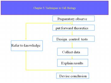
Chapter 3. Techniques in Cell Biology
Preparatory observe
put forward theoretics
Design control tests

Refer to knowledge
Collect data
Explain results
Devise conclusion
2
??????????????? ?????

• ???? ????
• ???? ??????
• ?? ??
• ??????????????????????
• (???????????)

3
?????????
???? ???? ??????? ????? ????? ?????? ?????
4
1.The Light Microscopy
5
A. Resolution and magnification
Figure 3-1. Resolving power. Sizes of cells and
their components drawn on a logarithmic scale,
indicating the range of objects that can be
readily resolved by the naked eye and in the
light and electron microscopes. The following
units of length are commonly employed in
microscopy µm (micrometer) 10-6 m nm
(nanometer) 10-9 m Å (Ångström unit) 10-10 m
6
Figure 3-2. Interference between light waves.
When two light waves combine in phase, the
amplitude of the resultant wave is larger and the
brightness is increased. Two light waves that are
out of phase partially cancel each other and
produce a wave whose amplitude, and therefore
brightness, is decreased.
7
Figure 3-3. Edge effects. The interference
effects observed at high magnification when light
passes the edges of a solid object placed between
the light source and the observer.
8
Figure 3-4. Numerical aperture. The path of light
rays passing through a transparent specimen in a
microscope, illustrating the concept of numerical
aperture and its relation to the limit of
resolution.
9
B. Preparation of specimen
??-??-??-??-??-??-??-??-??-??-??-??
Figure 3-5. Making tissue sections. How an
embedded tissue is sectioned with a microtome in
preparation for examination in the light
microscope.
10
(No Transcript)
11
C. Fluorescence Microscopy
Figure 3-7. The optical system of a modern
fluorescence microscope. A filter set consists of
two barrier filters (1 and 3) and a dichroic
(beam-splitting) mirror (2). In this example the
filter set for detection of the fluorescent
molecule fluorescein is shown.
12
                                         Figur
e 3-8. Fluorescent dyes. The structures of
fluorescein and tetramethylrhodamine, two dyes
that are commonly used for fluorescence
microscopy. Fluorescein emits green light,
whereas the rhodamine dye emits red light.
13
Figure 3-9. Fluorescence microscopy. Micrographs
of a portion of the surface of an early
Drosophila embryo in which the microtubules have
been labeled with an antibody coupled to
fluorescein (left panel) and the actin filaments
have been labeled with an antibody coupled to
rhodamine (middle panel). In addition, the
chromosomes have been labeled with a third dye
that fluoresces only when it binds to DNA (right
panel). At this stage, all the nuclei of the
embryo share a common cytoplasm, and they are in
the metaphase stage of mitosis. The three
micrographs were taken of the same region of a
fixed embryo using three different filter sets in
the fluorescence microscope.
14
D. Phase-contrast or a differential-interference-
contrast microscope
Figure 3-10. Two ways to obtain contrast in light
microscopy. The stained portions of the cell in
(A) reduce the amplitude of light waves of
particular wavelengths passing through them. A
colored image of the cell is thereby obtained
that is visible in the ordinary way. Light
passing through the unstained, living cell (B)
undergoes very little change in amplitude, and
the structural details cannot be seen even if the
image is highly magnified. The phase of the
light, however, is altered by its passage through
the cell, and small phase differences can be made
visible by exploiting interference effects using
a phase-contrast or a differential-interference-co
ntrast microscope.
15
                                                
                                          Figure
3-11. Four types of light microscopy. (A) The
image of a fibroblast in culture obtained by the
simple transmission of light through the cell, a
technique known as bright-field microscopy. The
other images were obtained by techniques
discussed in the text (B) phase-contrast
microscopy, (C) Nomarski differential-interference
-contrast microscopy, and (D) dark-field
microscopy.
16
E. Electronic image processing
Figure 3-12. Extending the limits of detection.
Light-microscope images of unstained microtubules
that have been visualized by differential-interfer
ence-contrast microscopy followed by electronic
image processing. (A) The original unprocessed
image. (B) The final result of an electronic
process that greatly enhances contrast and
reduces "noise." (Courtesy of Bruce Schnapp.)
17

• Video-enhance(contrast) microscopy

• Observing living specimens
• Greatly increase the contrast of an image so that
  very small objects become visible.

18
F. The confocal microscope
GFP can be used to study dynamic processes as
they occur in a living cell.
32.mov
32.mov
Figure 3-13. The confocal microscope. This
diagram shows that the basic arrangement of
optical components is similar to that of the
standard fluorescence microscope except that a
laser is used to illuminate a small pinhole whose
image is focused at a single point in the
specimen (A). Fluorescence from this focal point
in the specimen is focused at a second pinhole
(B). Light from elsewhere in the specimen is not
focused here and therefore does not contribute to
the final image (C). By scanning the beam of
light across the specimen, a very sharp
two-dimensional image of the exact plane of focus
is built up that is not significantly degraded by
light from other regions of the specimen.
19
Figure 3-14. Comparison of conventional and
confocal fluorescence microscopy. These two
micrographs are of the same intact gastrula-stage
Drosophila embryo that has been stained with a
fluorescent probe for actin filaments. The
conventional, unprocessed image (A) is blurred by
the presence of fluorescent structures above and
below the plane of focus. In the confocal image
(B), this out-of-focus information is removed,
which results in a crisp optical section of the
cell in the embryo.
20

2. Electron microscope
Figure 3-16. Limit of resolution of the electron
microscope. Electron micrograph of a thin layer
of gold showing the individual files of atoms in
the crystal as bright spots. The distance between
adjacent files of gold atoms is about 0.2 nm (2
Å).
21
(No Transcript)
22
I. Transmission Electron Microscopy
A. The comparison of the lens systems of LM and
TEM
23
A. Principal
Figure 3-17. Principal features of a light
microscope, a transmission electron microscope,
and a scanning electron microscope. These
drawings emphasize the similarities of overall
design. Whereas the lenses in the light
microscope are made of glass, those in the
electron microscope are magnetic coils.
24
B. Specimen Preparation for Electron Microscopy
Chemical fixation
Figure 3-18. Two common chemical fixatives used
for electron microscopy. The two reactive
aldehyde groups of glutaraldehyde enable it to
cross-link various types of molecules, forming
covalent bonds between them. Osmium tetroxide is
reduced by many organic compounds with which it
forms cross-linked complexes. It is especially
useful for fixing cell membranes, since it reacts
with the CC double bonds present in many fatty
acids.
25
Specimen Preparation for Electron Microscopy

• Thin Sectioning for TEM

The wax sections 3-10um The Plastic
ultrathin-sections for TEM 40-50nm
Sections of LM gt5um Sections of TEM lt100nm
26
Thin sections
                                         Figur
e 3-19. Diagram of the copper grid used to
support the thin sections of a specimen in the
transmission electron microscope.
27
Figure 3-20. Electron micrograph of a root-tip
cell stained with osmium and other heavy metal
ions. The cell wall, nucleus, vacuoles,
mitochondria, endoplasmic reticulum, Golgi
apparatus, and ribosomes are easily seen.
28
Figure 3-21. Electron micrograph of a cell
showing the location of a particular enzyme
(nucleotide diphosphatase) in the Golgi
apparatus. A thin section of the cell was
incubated with a substrate that formed an
electron-dense precipitate upon reaction with the
enzyme
29
Figure 3-63. Immunogold electron microscopy.
Electron micrographs of an insulin-secreting cell
in which the insulin molecules have been labeled
with anti-insulin antibodies bound to tiny
colloidal gold spheres. Most of the insulin is
stored in the dense cores of secretory vesicles
in addition, some cores are being degraded in
lysosomes.
30
                              Figure 3-22.
Three-dimensional reconstruction from serial
sections. Single thin sections sometimes give
misleading impressions. In this example most
sections through a cell containing a branched
mitochondrion will appear to contain two or three
separate mitochondria. Sections 4 and 7,
moreover, might be interpreted as showing a
mito-chondrion in the process of dividing. The
true three-dimensional shape, however, can be
reconstructed from serial sections.
31
II. Scanning electron microscope (SEM)
Images of surfaces can be obtained by
SEM Critical-point drying Range 15-150,000 X.
Resolution 5nm
32
Figure 3-23. Scanning electron microscopy.
Scanning electron micrograph of the stereocilia
projecting from a hair cell in the inner ear of a
bullfrog (A). For comparison, the same structure
is shown by differential-interference-contrast
light microscopy (B) and by thin-section electron
microscopy (C).
33
                                                
    Figure 3-32. Cells in culture. Scanning
electron micrograph of rat fibroblasts growing on
the plastic surface of a tissue-culture dish.
34
III. Metal Shadowing Allows Surface Features to
Be Examined
Figure 3-24. Electron micrographs of individual
myosin protein molecules that have been shadowed
with platinum. Myosin is a major component of the
contractile apparatus of muscle. As shown here,
it is composed of two globular head regions
linked to a common rodlike tail.
35
Figure 3-25. Preparation of a metal-shadowed
replica of the surface of a specimen. Note that
the thickness of the metal reflects the surface
contours of the original specimen.
36
IV. Freeze-Fracture and Freeze-Etch Electron
Microscopy
Figure 3-26. Freeze-fracture electron micrograph
of the thylakoid membranes from the chloroplast
of a plant cell. These membranes, which carry out
photosynthesis, are stacked up in multiple
layers. The largest particles seen in the
membrane are the complete photosystem II-a
complex of multiple proteins.
37
                                                
                                          Figure
3-27. Freeze-etch electron microscopy. The
specimen is rapidly frozen, and the block of ice
is fractured with a knife (A). The ice level is
then lowered by sublimation in a vacuum, exposing
structures in the cell that were near the
fracture plane (B). Following these steps, a
replica of the still frozen surface is prepared,
and this is examined in a transmission electron
microscope.
38

• Freeze Fracture
• Replication and
• Freeze Etching

quick freeze deep etching
39
Figure 3-28. Regular array of protein filaments
in an insect muscle. To obtain this image, the
muscle cells were rapidly frozen to liquid helium
temperature, fractured through the cytoplasm, and
subjected to deep etching. A metal-shadowed
replica was then prepared and examined at high
magnification. (Courtesy of Roger Cooke and John
Heuser.)
40
Quick-freeze, deep-etch electron microscopy of
processes in MAP2 (a), MAP2C (b) or tau (c)
transfected Sf9 cells, and microtubules
copolymerized in vitro with either MAP2 (d) or
tau (e).
41
V. Negative Staining and Cryoelectron Microscopy
Allow Macromolecules to Be Viewed at High
Resolution
Figure 3-29. Electron micrograph of negatively
stained actin filaments. Each filament is about 8
nm in diameter and is seen, on close inspection,
to be composed of a helical chain of globular
actin molecules. (Courtesy of Roger Craig.)
42
Figure 10-31. The three-dimensional structure of
a bacteriorhodopsin molecule. The polypeptide
chain crosses the lipid bilayer as seven a
helices. The location of the chromophore and the
probable pathway taken by protons during the
light-activated pumping cycle are shown. When
activated by a photon, the chromophore is thought
to pass an H to the side chain of aspartic acid
85 (pink sphere marked 85). Subsequently, three
other H transfers are thought to complete the
cyclefrom aspartic acid 85 to the extra-cellular
space, from aspartic acid 96 (pink sphere marked
96) to the chromophore, and from the cytosol to
aspartic acid 96. (R. Henderson et al. J. Mol.
Biol.213899-929)
43
3. Isolating Cells and Growing Them in Culture
44
Figure 3-31. A fluorescence-activated cell
sorter. When a cell passes through the laser
beam, it is monitored for fluorescence. Droplets
containing single cells are given a negative or
positive charge, depending on whether the cell is
fluorescent or not. The droplets are then
deflected by an electric field into collection
tubes according to their charge. Note that the
cell concentration must be adjusted so that most
droplets contain no cells and flow to a waste
container together with any cell clumps. The same
apparatus can also be used to separate
fluorescently labeled chromosomes from one
another, providing valuable starting material for
the isolation and mapping of genes.
45
Figure 3-32. Cells in culture. Scanning electron
micrograph of rat fibroblasts growing on the
plastic surface of a tissue-culture dish.
(Courtesy of Guenter Albrecht-Buehler.)
46
Figure 3-33. The production of hybrid cells.
Human cells and mouse cells are fused to produce
heterocaryons, which eventually form hybrid
cells. These particular hybrid cells are useful
for mapping human genes on specific human
chromosomes because most of the human chromosomes
are quickly lost in a random manner, leaving
clones that retain only one or a few. The hybrid
cells produced by fusing other types of cells
often retain most of their chromosomes.
47
4. The Fractionation and analysis for cells
contents
A. The technique of differential centrifugation
S(dx/dt)/?2x 1?10-13sec.
Step-by-step procedure for the purification of
organelles by differential centrifugation.
48
                                         Figu
re 3-34. The preparative ultracentrifuge.
49
Figure 3-35. Cell fractionation by
centrifugation. Repeated centrifugation at
progressively higher speeds will fractionate
homogenates of cells into their components. In
general, the smaller the subcellular component,
the greater is the centrifugal force required to
sediment it. Typical values for the various
centrifugation steps referred to in the figure
arelow speed 1,000 times gravity for 10 minutes
medium speed 20,000 times gravity for 20 minutes
high speed 80,000 times gravity for 1 hour very
high speed 150,000 times gravity for 3 hours
50
Figure 3-36. Comparison of methods of velocity
sedimentation and equilibrium sedimentation.
51
B. Paper chromatography
 Figure 3-37. The separation of small molecules
by paper chromatography. After the sample has
been applied to one end of the paper (the
"origin") and dried, a solution containing a
mixture of two or more solvents is allowed to
flow slowly through the paper by capillary
action. Different components in the sample move
at different rates in the paper according to
their relative solubility in the solvent that is
preferentially adsorbed onto the fibers of the
paper.
52
C. Column chromatography
Figure 3-38. The separation of molecules by
column chromatography. The sample is applied to
the top of a cylindrical glass or plastic column
filled with a permeable solid matrix, such as
cellulose, immersed in solvent. Then a large
amount of solvent is pumped slowly through the
column and is collected in separate tubes as it
emerges from the bottom. Various components of
the sample travel at different rates through the
column and are thereby fractionated into
different tubes.
53
Figure 3-39. Three types of matrices used for
chromatography. In ion-exchange chromatography
(A) the insoluble matrix carries ionic charges
that retard molecules of opposite charge.
Matrices commonly used for separating proteins
are DEAE-cellulose, which is positively charged,
and CM-cellulose and phosphocellulose, which are
negatively charged. In gel-filtration
chromatography (B) the matrix is inert but
porous. Molecules that are small enough to
penetrate into the matrix are thereby delayed and
travel more slowly through the column. Beads of
cross-linked polysaccharide (dextran or agarose)
are available commercially in a wide range of
pore sizes, making them suitable for the
fractionation of molecules of various molecular
weights, from less than 500 to more than 5 x 106.
Affinity chromatography (C) utilizes an insoluble
matrix that is covalently linked to a specific
ligand, such as an antibody molecule or an enzyme
substrate, that will bind a specific protein.
54
Figure 3-40. Protein purification by
chromatography. In this example a homogenate of
cells was first fractionated by allowing it to
percolate through an ion-exchange resin packed
into a column (A). The column was washed, and the
bound proteins were then eluted by passing a
solution containing a gradually increasing
concentration of salt onto the top of the column.
Proteins with the lowest affinity for the
ion-exchange resin passed directly through the
column and were collected in the earliest
fractions eluted from the bottom of the column.
The remaining proteins were eluted in sequence
according to their affinity for the resinthose
proteins binding most tightly to the resin
requiring the highest concentration of salt to
remove them. The fractions with activity were
pooled and then applied to a second,
gel-filtration column (B). The elution position
of the still-impure protein was again determined
by its enzymatic activity and the active
fractions pooled and purified to homogeneity on
an affinity column (C) that contained an
immobilized substrate of the enzyme.
55
D. SDS polyacrylamide-gel electrophoresis
Figure 3-41. The detergent sodium dodecyl sulfate
(SDS) and the reducing agent beta-mercaptoethanol.
These two chemicals are used to solubilize
proteins for SDS polyacrylamide-gel
electrophoresis. The SDS is shown here in its
ionized form.
56
Electrophoresis
Figure 3-42. SDS polyacrylamide-gel
electrophoresis (SDS-PAGE).
57
Figure 3-44. Separation of protein molecules by
isoelectric focusing. At low pH the carboxylic
acid groups of proteins tend to be uncharged (
-COOH) and their nitrogen-containing basic groups
fully charged ( -NH3), giving most proteins a
net positive charge. At high pH the carboxylic
acid groups are negatively charged (-COO-) and
the basic groups tend to be uncharged ( -NH2),
giving most proteins a net negative charge. At
its isoelectric pHa protein has no net charge
since the positive and negative charges balance.
Thus, when a tube containing a fixed pH gradient
is subjected to a strong electric field in the
appropriate direction, each protein species
present will migrate until it forms a sharp band
at its isoelectric pH, as shown.
58
Figure 3-45. Two-dimensional polyacrylamide-gel
electrophoresis. All the proteins in an E. coli
bacterial cell are separated in this gel, in
which each spot corresponds to a different
polypeptide chain. Note that different proteins
are present in very different amounts. The
bacteria were fed with a mixture of
radioisotope-labeled amino acids and the result
was detected by auto-radiography. (Courtesy of
Patrick O'Farrell.)
59
E. Western blotting or immunoblotting
Figure 3-46. Western blotting or immunoblotting.
The total proteins from dividing tobacco cells in
culture are first separated by two-dimensional
polyacrylamide-gel electrophoresis as shown in
and their positions revealed by a sensitive
protein stain (A). The separated proteins on an
identical gel were then transferred to a sheet of
nitrocellulose and incubated with an antibody
that recognizes those proteins that, during
mitosis, are phosphorylated on threonine
residues. The positions of the dozen or so
proteins that are recognized by this antibody are
revealed by an enzyme-linked second antibody (B).
(From J.A. Traas et al., Plant Journal2723-732)
60
(No Transcript)
61
Figure 3-47. Production of a peptide map, or
fingerprint, of a protein. Here, the protein was
digested with trypsin to generate a mixture of
polypeptide fragments, which was then
fractionated in two dimensions by electrophoresis
and partition chromatography. The pattern of
spots obtained is diagnostic of the protein
analyzed.
62
5. Protein structure
A. X-ray crystallography
Figure 3-48. X-ray crystallography. (A) Protein
crystal of ribulose bisphosphate carboxylase, an
enzyme that plays a central role in CO2 fixation
during photosynthesis. (B) X-ray diffraction
pattern obtained from the crystal. (C) Simplified
model of the protein structure derived from the
x-ray diffraction data. (A, courtesy of C.
Branden B, courtesy of J. Hajdu and I.
Andersson C, adapted from original provided by
B. Furugren.)
63
B. NMR spectroscopy
Figure 3-49. NMR spectroscopy. (A) An example of
the data from an NMR machine. This is a
two-dimensional NMR spectrum derived from the
carboxyl-terminal domain of the enzyme cellulase.
The spots represent interactions between hydrogen
atoms that are near neighbors in the protein and
hence their distance apart. Complex computing
methods, in conjunction with the known amino acid
sequence, enable possible compatible structures
to be derived. In (B) 10 structures, which all
satisfy the distance constraints equally well,
are shown superimposed on one another, giving a
good indication of the probable three-dimensional
structure. (Courtesy of P. Kraulis.)
64
6. Tracing and Assaying Molecules Inside Cells
Figure 7-20. In situ hybridization for RNA
localization in tissues. Autoradiograph of a
section of a very young Drosophila embryo that
has been subjected to in situ hybridization using
a radioactive DNA probe complementary to a gene
involved in segment development. The probe has
hybridized to RNA in the embryo, and the pattern
of autoradiographic silver grains reveals that
the RNA made by the gene (ftz) is localized in
alternating stripes across the embryo that are
three or four cells wide. At this stage of
development (cellular blastoderm), the embryo
contains about 6000 cells. (E. Hafen et al, Cell
37833-841, 1984.)
65
Figure 3-51. Electron-microscopic
autoradiography. The results of a pulse-chase
experiment in which pancreatic beta cells were
fed 3H-leucine for 5 minutes followed by excess
unlabeled leucine (the chase). The amino acid is
largely incorporated into insulin, which is
destined for secretion. After a 10-minute chase
the labeled protein has moved from the rough ER
to the Golgi stacks (A), where its position is
revealed by the black silver grains in the
photographic emulsion. After a further 45-minute
chase the labeled protein is found in
electron-dense secretory granules (B).(Courtesy
of L. Orci, from Diabetes 31538-565)
66
Figure 3-57. Visualizing intracellular Ca2
concentrations using a fluorescent indicator. The
branching tree of dendrites of the Purkinje cell
in the cerebellum receives more than 100,000
synapses from other neurons. The output from the
cell is conveyed along the single axon seen
leaving the cell body at the bottom of the
picture. This image of the intracellular calcium
concentration in a single Purkinje cell was taken
using a low-light camera and the Ca2-sensitive
fluorescent indictor fura-2. The concentration of
free Ca2 is represented by different colors, red
being the highest and blue the lowest. (Courtesy
of D.W. Tank et al.)
67
Figure 3-58. Fluorescent analogue cytochemistry.
Fluorescence micrograph of the leading edge of a
living fibroblast that has been injected with
rhodamine-labeled tubulin. The microtubules
throughout the cell have incorporated the labeled
tubulin molecules. Thus individual microtubules
can be detected and their dynamic behavior
followed using computer-enhanced imaging, as
shown here. Although the microtubules appear to
be about 0.25 µm thick, this is an optical
effect they are, in reality, only one-tenth this
diameter. (Courtesy of P. Sammeh and G. Borisy.)
68
Figure 3-59. Methods to introduce a
membrane-impermeant substance into a cell. (A)
the substance is injected through a micropipette.
(B) the cell membrane is made transiently
permeable to the substance by disrupting the
membrane structure with a brief but intense
electric shock. (C) membrane-bounded vesicles are
loaded with the desired substance and then
induced to fuse with the target cells.
69
Figure 3-64. Indirect immunocytochemistry. The
method is very sensitive because the primary
antibody is itself recognized by many molecules
of the secondary antibody. The secondary antibody
is covalently coupled to a marker molecule that
makes it readily detectable. Commonly used marker
molecules include fluorescein or rhodamine dyes,
the enzyme horseradish peroxidase or colloidal
gold spheres, and the enzymes alkaline
phosphatase or peroxidase.
70
7. Monoclonal Antibodies
Figure 3-65. Preparation of hybridomas that
secrete monoclonal antibodies against a
particular antigen (X). The selective growth
medium used contains an inhibitor (aminopterin)
that blocks the normal biosynthetic pathways by
which nucleotides are made. The cells must
therefore use a bypass pathway to synthesize
their nucleic acids, and this pathway is
defective in the mutant cell line to which the
normal B lymphocytes are fused. Because neither
cell type used for the initial fusion can grow on
its own, only the hybrid cells survive.
71
8. Gene Knockout mice
Mario Capecchi (Late 1980s) (University of
Utah) embryonic stem cells in inner cell mass as
target cells 1/104 cells undergo a process of
homologous recombination.
72
9. The technique for the take apart and gather
up of cell, and microscope manipulation

• Preparation and reform of karyoplast and
  cytoplast
• Transgenic animals and plants

Transgenic mice 10 weeks 44g and 29g
73
(No Transcript)
74
(No Transcript)
75
(No Transcript)
76
(No Transcript)
77
(No Transcript)
78
(No Transcript)
79
(No Transcript)
80
(No Transcript)
81
(No Transcript)
82
THANKS!