
Heat Transfer and Thermal Boundary Conditions PowerPoint PPT Presentation
1 / 27
Title: Heat Transfer and Thermal Boundary Conditions
1
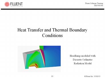
Heat Transfer and Thermal Boundary Conditions
- Headlamp modeled with
- Discrete Ordinates
- Radiation Model
2
Outline
- Introduction
- Thermal Boundary Conditions
- Fluid Properties
- Conjugate Heat Transfer
- Natural Convection
- Radiation
- Periodic Heat Transfer
3
Introduction
- Heat transfer in Fluent solvers allows inclusion
of heat transfer within fluid and solid regions
in your model. - Handles problems ranging from thermal mixing
within a fluid to conduction in composite solids.
- Energy transport equation is solved, subject to a
wide range of thermal boundary conditions.
4
Options
- Inclusion of species diffusion term
- Energy equation includes effect of enthalpy
transport due to species diffusion, which
contributes to energy balance. - This term is included in the energy equation by
default. - You can turn off the Diffusion Energy Source
option in the Species Model panel. - Term always included in the coupled solver.
- Energy equation in conducting solids
- In conducting solid regions, simple conduction
equation solved - Includes heat flux due to conduction and
volumetric heat sources within solid. - Convective term also included for moving solids.
- Energy sources due to chemical reaction are
included for reacting flow cases.
5
User Inputs for Heat Transfer (1)
- 1. Activate calculation of heat transfer.
- Select the Enable Energy option in the Energy
panel. - Define ? Models ? Energy...
- Enabling reacting flow or radiation will toggle
Enable Energy on without visiting this panel.
6
User Inputs for Heat Transfer (2)
- 2. To include viscous heating terms in energy
equation, turn on Viscous Heating in Viscous
Model panel. - Describes thermal energy created by viscous shear
in the flow. - Often negligible not included in default form of
energy equation. - Enable when shear stress in fluid is large (e.g.,
in lubrication problems) and/or in high-velocity,
compressible flows. - 3. Define thermal boundary conditions.
- Define ? Boundary Conditions...
- 4. Define material properties for heat transfer.
- Define ? Materials...
- Heat capacity and thermal conductivity must be
defined. - You can specify many properties as functions of
temperature.
7
Solution Process for Heat Transfer
- Many simple heat transfer problems can be
successfully solved using default solution
parameters. - However, you may accelerate convergence and/or
improve the stability of the solution process by
changing the options below - Underrelaxation of energy equation.
- Solve ? Controls ? Solution...
- Disabling species diffusion term.
- Define ? Models ? Species...
- Compute isothermal flow first, then add
calculation of energy equation. - Solve ? Controls ? Solution...
8
Theoretical Basis of Wall Heat Transfer
- For laminar flows, fluid side heat transfer is
approximated as - n local coordinate normal to wall
- For turbulent flows, law of the wall is extended
to treat wall heat flux. - The wall-function approach implicitly accounts
for viscous sublayer. - The near-wall treatment is extended to account
for viscous dissipation which occurs in the
boundary layer of high-speed flows.
9
Thermal Boundary Conditions at Flow Inlets and
Exits
- At flow inlets, must supply fluid temperature.
- At flow exits, fluid temperature extrapolated
from upstream value. - At pressure outlets, where flow reversal may
occur, backflow temperature is required.
10
Thermal Conditions for Fluids and Solids
- Can specify an energy source using Source Terms
option.
11
Thermal Boundary Conditions at Walls
- Use any of following thermal conditions at walls
- Specified heat flux
- Specified temperature
- Convective heat transfer
- External radiation
- Combined external radiation and external
convective heat transfer
12
Fluid Properties
- Fluid properties such as heat capacity,
conductivity, and viscosity can be defined as - Constant
- Temperature-dependent
- Composition-dependent
- Computed by kinetic theory
- Computed by user-defined functions
- Density can be computed by ideal gas law.
- Alternately, density can be treated as
- Constant (with optional Boussinesq modeling)
- Temperature-dependent
- Composition-dependent
13
Conjugate Heat Transfer
- Ability to compute conduction of heat through
solids, coupled with convective heat transfer in
fluid. - In 2D Cartesian coordinates
- Solid properties may vary with location, e.g.,
- Density, ?w
- Specific heat, cw
- Conductivity, kw
- Solid conductivity, kw, may also be function of
temperature. - is a uniformly distributed volumetric heat
source. - May be function of time and space (using profiles
or user-defined functions).
14
Conjugate Heat Transfer in Fuel-Rod Assembly
- Fluid flow equations not solved within solid
regions. - Energy equation solved simultaneously in full
domain. - Convective terms dropped in stationary solid
regions.
15
Natural Convection - Introduction
- Natural convection occurs when heat is added to
fluid and fluid density varies with temperature. - Flow is induced by force of gravity acting on
density variation.
16
Natural Convection - Boussinesq Model
- Makes simplifying assumption that density is
uniform. - Except for body force term in momentum equation,
which is replaced by - Valid when density variations are small.
- When to use Boussinesq model
- Essential to calculate time-dependent natural
convection inside closed domains. - Can also be used for steady-state problems.
- Provided changes in temperature are small
- You can get faster convergence for many
natural-convection flows than by using fluid
density as function of temperature. - Cannot be used with species calculations or
reacting flows.
17
User Inputs for Natural Convection (1)
- 1. Set gravitational acceleration.
- Define ? Operating Conditions...
- 2. Fluid density
- (a) If using Boussinesq model
- Select boussinesq as the Density method and
assign a constant value. - Set the Thermal Expansion Coefficient.
- Define ? Materials
- Set the Operating Temperature in the Operating
Conditions panel. - Define ? Operating Conditions...
- (b) Otherwise, define fluid density as function
of
temperature.
18
User Inputs for Natural Convection (2)
- 3. Optionally, specify Operating Density.
- Does not apply for Boussinesq model.
- 4. Set boundary conditions.
- Define ? Boundary Conditions...
19
Radiation
- Radiation intensity along any
direction
entering medium
is reduced by - Local absorption
- Out-scattering (scattering away
from the direction) - Radiation intensity along any
direction
entering medium is
augmented by - Local emission
- In-scattering (scattering into the direction)
- Four radiation models are provided in FLUENT
- Discrete Ordinates Model (DOM)
- Discrete Transfer Radiation Model (DTRM)
- P-1 Radiation Model
- Rosseland Model (limited applicability)
20
Discrete Ordinates Model
- The radiative transfer equation is solved for a
discrete number of finite solid angles - Advantages
- Conservative method leads to heat balance for
coarse discretization. - Accuracy can be increased by using a finer
discretization. - Accounts for scattering, semi-transparent media,
specular surfaces. - Banded-gray option for wavelength-dependent
transmission. - Limitations
- Solving a problem with a large number of
ordinates is CPU-intensive.
21
Discrete Transfer Radiation Model (DTRM)
- Main assumption radiation leaving surface
element in a specific range of solid angles can
be approximated by a single ray. - Uses ray-tracing technique to integrate radiant
intensity along each ray - Advantages
- Relatively simple model.
- Can increase accuracy by increasing number of
rays. - Applies to wide range of optical thicknesses.
- Limitations
- Assumes all surfaces are diffuse.
- Effect of scattering not included.
- Solving a problem with a large number of rays is
CPU-intensive.
22
P-1 Model
- Main assumption radiation intensity can be
decomposed into series of spherical harmonics. - Only first term in this (rapidly converging)
series used in P-1 model. - Effects of particles, droplets, and soot can be
included. - Advantages
- Radiative transfer equation easy to solve with
little CPU demand. - Includes effect of scattering.
- Works reasonably well for combustion applications
where optical thickness is large. - Easily applied to complicated geometries with
curvilinear coordinates. - Limitations
- Assumes all surfaces are diffuse.
- May result in loss of accuracy, depending on
complexity of geometry, if optical thickness is
small. - Tends to overpredict radiative fluxes from
localized heat sources or sinks.
23
Choosing a Radiation Model
- For certain problems, one radiation model may be
more appropriate in general. - Define ? Models ? Radiation...
- Computational effort P-1 gives reasonable
accuracy with
less effort. - Accuracy DTRM and DOM more accurate.
- Optical thickness DTRM/DOM for optically thin
media (optical
thickness ltlt 1) P-1 better for optically thick
media. - Scattering P-1 and DOM account for scattering.
- Particulate effects P-1 and DOM account for
radiation exchange between gas and particulates. - Localized heat sources DTRM/DOM with
sufficiently large number of rays/ ordinates is
more appropriate.
24
Periodic Heat Transfer (1)
- Also known as streamwise-periodic or
fully-developed flow. - Used when flow and heat transfer patterns are
repeated, e.g., - Compact heat exchangers
- Flow across tube banks
- Geometry and boundary conditions repeat in
streamwise direction.
Outflow at one periodic boundary is inflow at the
other
25
Periodic Heat Transfer (2)
- Temperature (and pressure) vary in streamwise
direction. - Scaled temperature (and periodic pressure) is
same at periodic boundaries. - For fixed wall temperature problems, scaled
temperature defined as - Tb suitably defined bulk temperature
- Can also model flows with specified wall heat
flux.
26
Periodic Heat Transfer (3)
- Periodic heat transfer is subject to the
following constraints - Either constant temperature or fixed flux bounds.
- Conducting regions cannot straddle periodic
plane. - Properties cannot be functions of temperature.
- Radiative heat transfer cannot be modeled.
- Viscous heating only available with heat flux
wall boundaries. - Flow must be specified by pressure jump in
coupled solvers.
Contours of Scaled Temperature
27
Summary
- Heat transfer modeling is available in all Fluent
solvers. - After activating heat transfer, you must provide
- Thermal conditions at walls and flow boundaries
- Fluid properties for energy equation
- Available heat transfer modeling options include
- Species diffusion heat source
- Combustion heat source
- Conjugate heat transfer
- Natural convection
- Radiation
- Periodic heat transfer
Recommended
