
Waves and Optics PowerPoint PPT Presentation
1 / 56
Title: Waves and Optics
1
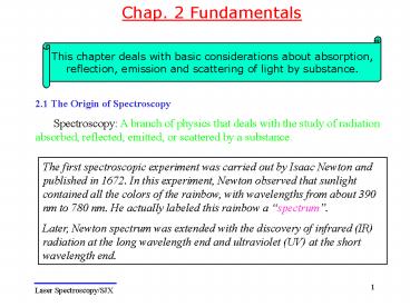
This chapter deals with basic considerations
about absorption, reflection, emission and
scattering of light by substance.
2.1 The Origin of Spectroscopy
Spectroscopy A branch of physics that deals with
the study of radiation absorbed, reflected,
emitted, or scattered by a substance.
The first spectroscopic experiment was carried
out by Isaac Newton and published in 1672. In
this experiment, Newton observed that sunlight
contained all the colors of the rainbow, with
wavelengths from about 390 nm to 780 nm. He
actually labeled this rainbow a
spectrum. Later, Newton spectrum was extended
with the discovery of infrared (IR) radiation at
the long wavelength end and ultraviolet (UV) at
the short wavelength end.
2
2.2 The Electromagnetic Spectrum and Optical
Spectroscopy
3
The electromagnetic spectrum is traditionally
divided into seven well-known spectral regions
radio waves, microwaves, infrared, visible and
ultraviolet light, X-rays, and ?-rays. All of
these radiation have in common the fact that they
propagate through the space as transverse
electromagnetic waves and at the same speed,
(2.1)
in vacuum. The various spectral regions of the
electromagnetic spectrum differ in wavelength and
frequency, which leads to substantial differences
in their generation, detection, and interaction
with matter. Each type of monochromatic
electromagnetic radiation is usually labeled by
its frequency ?, wavelength ?, photon energy ?,
or wavenumber . Their magnitudes are
interrelated by the well known quantization
equation
(2.2)
4
Figure 2.1 The electromagnetic spectrum, showing
the different microscopic excitation sources and
the spectroscopies related to the different
spectral regions. XRFX-ray fluorescence
AEFSabsorption edge fine structure
EXAFSExtended X-Ray absorption fine structure
NMRNuclear magnetic resonance EPRElectron
paramagnetic resonance. The shaded region
indicates the optical range. Microwaves are used
in magnetic resonance techniques (NMR and EPR) in
order to induce transitions between different
nuclear spin states or electron spin states.
The vibration frequencies of atoms in solids
are within the infrared frequency region.
Infrared absorption and Raman scattering are the
most relevant vibrational spectroscopic
techniques. Electronic energy levels are
separated by a wide range of energy values about
1-6 eV. These electrons are commonly called
valence electrons. They can be excited with
appropriate UV, VIS, or even near IR radiation in
a wavelength
5
range from about 200 nm to about 3000 nm. This
wavelength is called the optical range, and it
gives rise to optical spectroscopy. Inner
electrons of atoms are usually excited by X-rays.
Atoms give characteristic X-ray absorption and
emission spectra, due to a variety of ionization
and possible inter-shell transitions. Two
relevant refined X-ray absorption techniques,
that use synchrotron radiation, are the so-called
absorption Edge Fine Structure (AEFS) and
Extended X-ray Absorption Fine Structure (EXAFS).
These techniques are very useful in the
investigation of local structures in solids. On
the other hand, X-Ray Fluorescence (XRF) is an
important analytical technique. X-rays are used
in Mössbauer spectroscopy. It provides
information on the oxidation state, coordination
number, and bond character.
6
In this course, we shall focus on the Laser
Spectroscopy.
7
Four possible optical processesIf a solid
sample is illuminated by a light beam of
intensity I0, the intensity of this beam is
attenuated after it passes through the sample.
- Absorption. Makes electron transition from the
ground state to the excited states. - Luminescence. The electrons excited by light
absorption return to the ground state via
emitting light radiation. - Refection with an intensity IR from the external
and internal surfaces. - Scattering, with a light intensity IS spread in
several directions, due to elastic (at the same
frequency as the incident beam) or inelastic
scattering (at lower and higher frequencies than
that of the incident beamRaman scattering)
processes.
8
Colors and wavelength range
9
Laser Spectroscopy (absorption, luminescence,
reflection, and Raman scattering) analyzes the
frequency and intensity of these emerging beams
as a function of the frequency and intensity of
the incident laser beam. By means of laser
spectroscopy, we can understand the optical
properties and electronic structures of an
object. Experimental spectra are usually
presented as plots of the intensity of (absorbed,
emitted, reflected, or scattered) radiation
versus the photon energy (in eV), the wavelength
(in nm) or the wavenumber (in cm-1).
(2.3)
10
2.3 Absorption
2.3.1 Absorption Coefficient In the previous
section, we have mentioned that a light beam
becomes attenuated after passing through a
material. Experiments show that the beam
intensity attenuation dI after traversing a
differential thickness dx can be written as
where I is the light intensity at a distance x
into the material and a is called the absorption
coefficient of the material. Upon integration of
Eq. (2.4) we obtain which gives an exponential
attenuation law relating the incoming light
(2.4)
(2.5)
11
intensity I0 (Actually it is the incident
intensity minus the reflection losses at the
material surface) to the thickness x. This Law is
known as the Lambert-Beer law. From a
microscopic point of view of the absorption
process, we can assume a simple two energy level
quantum system for which N and N are the ground
state and excited state population densities (the
atoms per unit volume in each state). The
absorption coefficient of this system
can be written as where s(v) is the so-called
transition cross section. For low-intensity
incident beams, which is the usual situation in
light absorption experiments, NN and then Eq.
(2.6) can be written as
(2.6)
12
where the transition cross section s(v)
(normally given in cm2) represents the ability of
our system to absorb the incoming radiation with
frequency v . Indeed, the transition cross
section is related to the transition matrix
element of our two-level system,
where ?i and ?f denote the eigenfunctions of the
ground and excited states, respectively, and H
is the interaction Hamiltonian between the
incoming light and the system. Eq. (2.7) also
shows that the absorption coefficient is
proportional to the density of absorbing atoms
(or centers), N (normally expressed in cm-3).
For our two-level system, we should expect an
absorption spectrum like a d-function at a
frequency v0(E2-E1)/h, E2 and E1 being the
excited and ground state energies, respectively.
However, various line-broadening mechanisms
always exist in the real physical systems. So,
the observed spectrum never consists of a single
line, but of a band.
(2.7)
13
- An ideal absorption spectrum for a two-level
system. - The Lorentzian line shape of an optical
absorption band, related to homogeneous
broadening - The Gaussian line shape of an optical absorption
band, related to inhomogeneous broadening.
14
In fact, the transition cross section s(v) can be
written in terms of a line-shape function g(v)
(with units of Hz-1) in the following way where
is the so-called
transition strength. The line-shape function
g(v) gives the profile of the optical absorption
(and emission) band and contains important
information about the light-matter interaction.
Now let us briefly discuss the different
mechanisms that contribute to this function, or
the different line-broadening mechanisms. The
ultimate (minimum) linewidth of an optical band
is due to the natural or life-time broadening.
This broadening arises from the Heisenbergs
uncertainty principle, ?v?t1/2p, ?v being the
full frequency width at half maximum of the
transition and ?t the time available to measure
the frequency of the transition (basically, the
lifetime of the excited state). This broadening
mechanism leads to a
(2.8)
15
Lorentzian profile given by The natural
broadening is a type of homogeneous broadening,
in which all the absorbing atoms are assumed to
be identical and then to contribute with
identical line-shape function to the spectrum.
There are other homogeneous broadening
mechanisms, such as due to scattering of lattice
vibrations (phonons) in solids. EXAMPLE An
allowed emission transition for a given optical
ion in a solid has a lifetime of 10 ns. Estimate
its natural broadening. Then estimate the peak
value of g(v). According to Heisenbergs
uncertainty principle,
(2.9)
16
Due to natural broadening, the line shape of the
absorption spectrum should have a Lorentzian
profile described by Eq. (2.9), with a full
frequency width at half maximum of ?v16 MHz.
Now using Eq. (2.9), we can determine the peak
value for the line-shape function of the
transition In various cases, the different
absorbing centers have different resonant
frequencies, so that the line shape results from
the convolution of the line shapes of the
different centers, weighted by their
corresponding concentrations. Say this type of
broadening inhomogeneous broadening. In
general, inhomogeneous broadening leads to a
Gaussian line shape given by the expression
(2.10)
17
In the more general case, the line shape of a
given transition is due to the combined effect of
more than one independent broadening mechanism.
In this case, the overall line shape is given by
the convolution of the line-shape functions
associated with the different broadening
mechanisms. 2.3.2 Measurements of Absorption
Spectra the Spectrophotometer Absorption spectra
are usually registered by instruments known as
Spectrophotometers. The following figure shows a
schematic diagram with the main elements of the
simplest spectrophotometer (a single-beam
spectrophotometer). Basically, it consists of
these elements (1) a light source (usually a
deuterium lamp for the UV spectral range and a
tungsten lamp for the VIS and IR spectral range)
that is focused on the entrance to (2) a
monochromator, which is used to select a single
frequency (wavelength) from all of those provided
by the lamp source and to scan over a desired
frequency range (3) a sample holder, followed by
(4) a photodetector (usually a photomultiplier
for the UV-
18
Schematic diagram of a single-beam
spectrophotometer and (b) a double-beam
spectrophotometer.
19
VIS range and a PbS cell for the IR range) to
measure the intensity of each monochromatic beam
after traversing the sample and finally (5) a
computer, to display and record the absorption
spectrum. Optical spectrophotometer work in
different modes to measure optical density,
absorbance, or transmittance. The optical density
is defined as ODlog(I0/I), so that according to
Eq. (2.5) the absorption coefficient is
determined by That is, by measuring the optical
density and the sample thickness, the absorption
coefficient can be determined. According to Eq.
(2.7) we can now determine the absorption cross
section if the density of centers is known. On
the other hand, if the absorption cross section
is known, the concentration of absorbing centers,
N , can be estimated. The optical density can be
easily related to other well-known optical
(2.11)
20
magnitudes that are also directly measurable by
spectrophotometers, such as the transmittance,
TI/I0, and the absorbance, A1-I/I0
Nevertheless, it is important to emphasize
here the advantage of measuring optical density
spectra over transmittance or absorbance spectra.
Optical density spectra are more sensitive, as
they provide a higher contrast than absorbance or
transmittance spectra. In fact, for low optical
densities, expression (2.12) gives A1-(1-OD)OD,
so that the absorbance spectrum (A versus ?, or
1-T versus ?) displays the same shape as the
optical density. However, for high optical
densities, typically higher than 0.2, the
absorbance spectrum gives a quite different shape
to that of the actual absorption spectrum
(aversus ? or OD versus ?).
(2.12)
21
A single-beam spectrophotometer presents a
variety of problems, because the spectra are
affected by spectral and temporal variations in
the illumination intensity. The spectral
variations are due to the combined effects of the
lamp spectrum and the monochromator response,
while the temporal variations occur because of
lamp stability. To reduce these effects,
double-beam spectrophotometers are used. In the
previous figure, a schematic diagram of the main
components of the double-beam spectrophotometer.
The illuminating beam is spilt into two beams of
equal intensity, which are directed toward two
different channels a reference channel and a
sample channel. The outgoing intensities
correspond to I0 and I, respectively, which are
detected by two similar detectors, D1 and D2. As
a consequence, the spectral and temporal
intensity variations of the illuminating beam
affect both the reference and sample beams in the
same way, and these effects are minimized in the
resulting absorption. Typical sensitivities of
(OD)min 5 10-3 can be achieved with these
spectrophotometers.
22
EXAMPLE If the cross section for a given
transition of Nd3 ions in a particular crystal
is 10-19 cm2 and a sample of thickness 0.5 mm is
used, determine the minimum concentration of
absorbing ions that can be detected with a
typical double-beam spectrophotometer. For a
typical double-beam spectrophotometer, the
sensitivity in terms of the optical density is
(OD)min 5 10-3. Therefore, using Eqs. ( 2.7)
and (2.11), the minimum concentration of
absorbing centers that can be detected is
Crystals have typical constituent concentration
of about 1022 cm-3, so that the previous minimum
concentration of Nd3 ions correspond to about
0.01 or 100 parts per million (ppm).
23
2.3.3 Reflectivity Reflectivity spectra provide
similar and complementary information to the
absorption measurements. For instance, absorption
coefficients corresponding to the fundamental
absorption are as high as 105-106 cm-1, so that
they can only be measured by using very thin
samples (thin films). In these cases, the
reflectivity spectra R(v) can be very
advantageous, as they manifest the singularities
caused by the absorption process but with the
possibility of bulk samples. In fact, the
reflectivity, R(v), and the absorption spectra,
a(v) , can be interrelated by using the so-called
Kramers-Krönig relations. The reflectivity at
each frequency is defined by where IR is the
reflected intensity. Reflectivity spectra can
be registered in two different modes (i) direct
(2.13)
24
(No Transcript)
25
- reflectivity or (ii) diffuse reflectivity. Direct
reflectivity measurements are made with
well-polished samples at normal incidence.
Diffusion reflectivity is generally used for
unpolished or powdered samples. The figure shown
in last slide shows the experimental arrangements
for measuring both types of spectra. - For direct reflectivity measurements,
monochromatic light (produced by a lamp and
monochromator) is passed through a
semitransparent lamina (the beam splitter). This
lamina deviates the light reflected from the
sample toward a detector. - For diffuse reflectivity measurements, an
integrating sphere ( a sphere with a fully
reflective inner surface is used. Such a sphere
has a pinhole through which the light enters and
is transmitted toward the sample. the diffuse
reflected light reaches the detector after
suffering multiple reflections in the inner
surface of the sphere. The integrating spheres
can be incorporated as additional instrumentation
into conventional spectrophotometers.
26
2.4 Luminescence
Luminescence is, in some ways, the inverse
process to absorption. However, the absorption of
light is only one of the multiple mechanisms by
which a system can be excited. In a general
sense, luminescence is the emission of light from
a system that is excited by some of energy. Table
1.2 lists the most important types of
luminescence according to the excitation
mechanism.
27
Photoluminescence occurs after excitation with
light (i.e., radiation within the optical range).
Luminescence can also be produced under
excitation with an electron beam, and in this
case it is called cathodoluminescence. Excitation
by high-energy electromagnetic radiation
(sometimes called ionizing radiation) such as
X-rays, a-rays (helium nuclei), ß-rays
(electrons), or ?-rays leads to a type of
photoluminescence called radioluminescence.
Thermoluminescence occurs when a substance emits
light as a result of the release of energy stored
in traps by thermal heating. Electroluminescence
occurs as a result of the passage of an electric
current through a material. Triboluminescence is
the production of light by a mechanical
disturbance. Acoustic waves (sound) passing
through a liquid can produce sonoluminescence.
28
Chemiluminescence appears as a result of a
chemical reaction. As a particular class of
chemiluminescence, bioluminescence occurs as a
result of chemical reactions inside an organism.
Bioluminescence is the predominant source of
light in the deep ocean. 2.4.1 Measurement of
Photoluminescence Spectrofluorimeter We will now
focus our attention on the photoluminescence (PL
in short.) process. A typical experimental
arrangement to measure PL spectra is sketched in
the following figure.
29
PL spectrum measurement setup is usually called
spectrofluorimeter. The sample is excited
with a lamp, which is followed by a monochromator
(the excitation monochromator) or a laser beam.
The emitted is collected by a focusing lens and
dispersed by means of a second monochromator (the
emission monochromator), followed by a sutiable
detector connected to a computer. Two kinds of
spectra, (i) emission spectra and (ii) excitation
spectra, can be registered (i) In emission
spectra, the excitation wavelength is fixed and
the emitted light intensity is measured at
different wavelength by scanning the emission
monochromator. (ii) In excitation spectra, the
emission monochromator is fixed at an emission
wavelength while the excitation length is scanned
in a certain spectral range. The difference
between emission and excitation spectra can be
better understood with the aid of next example.
30
EXAMPLE Consider a phosphor with a three energy
level scheme and the absorption spectrum shown in
the following figure (a). Assuming similar
transition probabilities among these levels,
discuss the nature of the excitation and emission
spectra and their relationship to the absorption
spectrum. The absorption spectrum shows two
bands at photon energies hv1 and hv2,
corresponding to the 0?1 and 0?2 transitions,
respectively. Let us first discuss on the
possible emission spectra. Excitation with light
of energy hv1 promotes electrons from the ground
state 0 to the excited state 1, which becomes
populated. Thus, the emission spectrum consists
of a single band centered at hv1. On the other
hand, when the excitation energy is fixed at hv2,
the emission spectrum may have three emission
bands that peak at energies of h(v2-v1), hv1, and
hv2, related to the transitions 2?1, 1?0, and
2?0, respectively. Let us now discuss the
different excitation spectra. If we were to set
the emission monochromator at a fixed energy
h(v2-v1), and scan the excitation monochromator,
we would obtain an excitation spectrum
31
consisting of only one peak at hv2. On the other
hand, when the emission monochromator is fixed at
hv1, the excitation spectrum will resemble the
absorption spectrum.
32
2.4.2 Luminescence Efficiency We know that the
photoluminescence can occur after a material
absorbs light. Thus, considering that an
intensity I0 enters the material and an intensity
I passes out of it, the emitted intensity Iem
must be proportional to the absorbed intensity
that is, Iem ? I0-I. In general, it is written as
Iem
?(I0-I) (2.14) where
the intensities are given in photons per second
and ? is called the luminescence efficiency or
the quantum efficiency. Defined in such a way,
the luminescence quantum efficiency represents
the ratio between the emitted and absorbed
photons and it can vary from 0 to 1. In a PL
experiment, actually only a fraction of the total
emitted light is measured. This fraction depends
on the collecting system and on the geometric
characteristics of the detector. Therefore, in
fact, the measured emitted intensity Iem can be
written in terms of the incident intensity as
Iem kg ?I0(1-10 -(OD))
(2.15)
33
where kg is a geometric factor that depends on
the experimental setup (the arrangement of the
optical components and the detector size) and OD
is the optical density of the sample. For low
optical excitation intensities, Eq. (2-15)
becomes Iem kg ?I0
((OD)) (2.16) It is clear
from above equation that the emitted intensity is
linearly dependent on the incident intensity and
is proportional to both the quantum efficiency
and the optical density (this only for low
optical densities). A quantum efficiency of ?indicates that a fraction of the absorbed energy
is lost by nonradiative processes. Normally,
these processes lead to sample heating. EXAMPLE
The sensitivity of luminescence. Consider a
photoluminescence experiment in which the
excitation source provides a power of 100 µW at a
wavelength of 400 nm. The luminescent sample can
absorb the light at this wavelength and emit
light with a quantum efficiency of ?0.1.
Assuming that kg 10-3 and a minimum
34
detectable luminescence intensity of 103 photons
per second, determine the minimum optical
intensity that can be detected by
luminescence. Each incident photon has an energy
of Therefore, the
incident intensity is The minimum optical
density, (OD)min, detectable with our PL setup
can be obtained from Eq. (2.16)
35
Comparing this value to the typical sensitivity
provided by a spectrophotometer, (OD)min 5 x
10-3, we see that the luminescence technique is
much more sensitive than the absorption technique
(about 105 times for this experiment). 2.4.3
Stokes and Anti-Stokes Shifts Up to now, we have
considered that, for our simple two-level system,
the absorption and emission spectra peak at the
same energy. In fact, this is not true.
Generally, the emission spectrum is shifted to
lower energies relative to the absorption
spectrum. Such a shift is called Stokes shift.
We now give a simple explanation for it. Let us
consider that the two-level system shown in the
following figure (Fig. (a)) corresponds to an
optical ion embedded in an ionic crystal. These
two energy levels are a consequence of the
optical ion and its neighbors ions being at
fixed positions (rigid lattice). However, we
know that ions in solids are vibrating around
their equilibrium positions, so that our optical
ion see the neighbors at different distances,
oscillating around equilibrium positions.
Consequently, we must consider the role of
36
the neighboring ions in the optical transition of
the two-energy levels. To do so, we assume a
single coordinate distance Q, and that
neighboring ions follow a harmonic oscillation.
The two energy levels will become parabolic bands
as in the Fig. (b). In the spirit of this
approach, we will justify our claim that the
equilibrium positions of the ground and excited
states can be different and that the electronic
transitions occur as shown in the Fig. (b). Four
steps can be considered. First, an electron in
the ground state is
37
promoted to the excited state without any change
in Q0 (the equilibrium position in the ground
state). Afterwards, the electron relaxes within
the electronic states to its minimum position
Q0, its equilibrium position in the excited
state. This relaxation is a nonradiative process
accompanied by phonon emissions. From this
equilibrium Q0, luminescence is produced from
jumping down of the electron from the excited
state to the ground state, without any change in
the distance coordinate, QQ0. Finally, the
electron relaxes within the electronic states
again to the minimum of the ground state with the
equilibrium position Q0. As a result of these
four processes, the emission occurs at a
frequency vem, which is lower than vabs. The
energy difference ? hvabs-hvem is a measure of
the Stokes shift. Once the Stokes shift has
been introduced, we can better understand the
definition of luminescence quantum efficiency in
terms of absorbed and emitted photons per second
rather than the absorbed and emitted intensity
(the energy per second per unit area). In fact,
it is possible to have a system for which ?1
but, because of the Stokes shift, the emitted
energy can be lower than the absorbed energy. The
fraction of the absorbed energy that is not
emitted is delivered as phonons to the crystal
lattice (heating the sample).
38
It is also possible to obtain luminescence at
photon energies higher than the absorbed photon
energy. This is called anti-Stokes or
up-conversion luminescence and it occurs for
multilevel systems, as in the example shown in
the figure.
For this system, two photons of frequency vabs
are sequentially absorbed from the ground state 0
and then from the first excited state 1, thus
prompting an electron to the excited state 3.
Then, the electron decays nonradiatively to state
2, from which the anti-Stokes luminescence 2?0 is
produced. We thus observe the emission at
frequency vem vabs.
39
Note that anti-Stokes luminescence is, in
general, a nonlinear process. It is not difficult
to show that the intensity of the anti-Stokes
luminescence varies with the square of the
excitation intensity. 2.4.4 Time-Resolved
Luminescence In the previous sections, we have
considered the condition of continuous wave
excitation (i.e., the excitation intensity is
kept constant at each wavelength). This situation
corresponds to the stationary case, in which the
optical feeding into the excited level equals the
decay rate to the ground state and so the emitted
intensity remains constant with time. Now we
consider the sample under pulsed wave excitation.
This type of excitation prompts a nonstationary
density of centers N in the excited state. These
excited centers can decay to the ground state by
radiative (light-emitting) and nonradiative
processes, giving a decay-time intensity signal.
The temporal evolution of the excited state
population follows a very general rule
40
(2.17)
where AT is the total decay rate (or total decay
probability), which is written as
(2.18)
Here A is the radiative rate (the Einstein
coefficient of spontaneous emission) and Anr is
the nonradiative rate for the nonradiative
processes. The solution of the differential
equation (2.17) gives the density of excited
centers at any time t
(2.19)
where N0 is the population density of excited
centers at t0. The de-excitation process can
be experimentally observed by analyzing the
temporal decay of the emitted light. In fact, the
emitted light intensity at a given time t,
Iem(t), is proportional to the density of
41
centers de-excited per unit time,
(dN/dt)radiative AN(t), so that it can be
written as
(2.20)
where C is a proportionality constant and so I0
CAN0 is the emission intensity at t0. Equation
(2.20) corresponds to an exponential decay law
for the emitted intensity, with a lifetime given
by t 1/AT . This lifetime represents the time in
which the emitted intensity decays to I0/e and it
can be obtained from the slope of the linear
plot, logI versus t. As t is measured from a
pulsed luminescence experiment, it is called
fluorescence or luminescence lifetime. It is
important to stress that this lifetime value
gives the total decay time (radiative plus
nonradiative rates). Consequently Eq. (2.18) is
usually written as
(2.21)
where t0 is the so-called radiative lifetime. In
general case t 42
the nonradiative rate differs from zero. The
quantum efficiency ? can now be expressed in
terms of the radiative t0 and luminescence t
lifetimes
(2.22)
This equation indicates that the radiative
lifetime t0 can be determined from luminescence
decay-time measurements if the quantum efficiency
? is measured by an independent experiment.
EXAMPLE The luminescence lifetime measured
from the metastable state 4F3/2 of Nd3 ions in
the laser crystal yttrium aluminum borate
(YAl3(BO3)4) is 56 µs. If the quantum efficiency
from this state is 0.26, determine the radiative
lifetime and the radiative and nonradiative
rates. According to Eq. (2.22), the radiative
lifetime t0 is
43
and therefore the radiative rate is given by
The total de-excitation rate AT is So
that the nonradiative rate is The
nonradiative rate is much higher than the
radiative rate as a result, noticeable
pump-induced heating effect occurs in this laser
crystal. Time-resolved luminescence spectra
The emission spectra can also be recorded at
different times after the excitation pulse has
44
Schematic diagram of a typical time-resolved
photoluminescence system based on Streak-Camera
technique.
45
been absorbed. This experimental procedure is
called time-resolved luminescence and may prove
to be of great utility in the understanding of
complicated emitting systems. The figure in last
slide shows a schematic diagram of time-resolved
PL system based on Streak-Camera technique. The
fundamental principle of streak-camera will be
discussed in Chap. 4. The basic idea of the
time-resolved PL technique is to record the
emission spectrum at a certain delay time, t, in
respect to the excitation pulse and within a
temporal gate,?t, as schematically shown in the
following figure.
46
Thus, for different delay times different
spectral shapes are obtained.
Measured time-resolved PL spectra of ZnO at 77 K.
47
2.5 Rayleigh and Raman Scattering
After discussing light absorption, reflectance,
and emission in the previous sections, now let us
deal with the study of the fraction of light
scattered from incident light. A common
manifestation of light scattering is the red
color of the sky during day or night breaks, or
the blue sky during the day. Both occur as a
result of Rayleigh scattering of the sunlight due
to molecules in the atmosphere. This type of
scattering is an elastic photon process in which
the frequency of scattered light keeps
unchanged. Inelastic photon scattering processes
are also possible. In 1928, the Indian scientist
C. V. Raman demonstrated a type of inelastic
light scattering that had already been predicted
by A. Smekal in 1923. Raman won the Nobel Prize
in 1930. This type of scattering gives rise to a
new type of spectroscopy, Raman spectroscopy, in
which the light is inelastically scattered by a
substance. That is, the frequency of scattered
light is different from that of the incident
light.
48
Following figure shows how the Raman effect is
manifested spectrally. When light (usually laser
light) of frequency ?0 comes in over the sample,
the output spectrum of scattered light consists
of a predominant
line of the same frequency ?0 and much weaker (
1/1000 of the main band) side bands at
frequencies ?0Oi . The main line corresponds to
the Rayleigh scattered light , while side-band
spectrum is the actual Raman spectrum. Raman
spectrum has the following particular properties
49
- The Oi are the characteristic frequencies of the
substance (in case of solids, they correspond to
phonon frequencies). - Stokes and anti-Stokes lines are always at
frequencies located that are symmetrically to
both sides of the main line (Rayleigh line) at
?0. - The anti-Stokes lines are weaker than the Stokes
lines. - The intensity of the Raman lines is proportional
to ?04.
Raman spectra are usually represented by the
intensity of Stokes lines versus the shifted
frequencies Oi , as shown in the following
figure.
50
Most of the four above-mentioned properties for
Raman spectra can be explained by using a simple
classical model. When the crystal is subject to
the oscillating electric field of the
incident electromagnetic radiation, it becomes
polarized. In the linear approximation, the
induced electric polarization in any specific
direction is given by where
is the susceptibility tensor. As for other
physical properties of the crystal, the
susceptibility becomes altered because the atoms
in the solid are vibrating periodically around
equilibrium positions. Thus, for a particular
vibrating mode (phonon) at frequency O, each
component of the susceptibility tensor can be
expressed as where
represents a normal coordinate measured from the
equilibrium position. Therefore, using Eq.
(2.23), the induced polarization can be written as
(2.23)
51
where we have denoted .
This expression corresponds to oscillating
dipoles re-radiating light at frequencies of ?0
(Rayleigh light), ?0-O (Stokes Raman light), and
?0O (anti-Stokes Raman light). This explains the
appearance of the Raman lines at symmetric
frequencies in respect to ?0, as stated in points
(1) and (2) above. On the other hand, the
radiated intensity of such oscillating dipoles is
proportional to , so that we
can write The first term on the right-hand
side of Eq. (2.25) accounts for the generated
intensity due to Rayleigh scattered light, while
the second term is related to the intensity of
the Raman scattered light. For visible light ?0
1015 Hz, while the characteristic phonon
frequencies are
(2.24)
(2.25)
52
much smaller, typically O 1012 Hz. Thus ?s4
?04 , and the intensity of Raman scattering
varies as ?04 , as stated in point (4) above.
However, the classic model can not explain the
property (3) of the Raman effect. Property (3)
can also be regarded from a quantum mechanical
viewpoint by using the energy-level scheme as
shown in the following figure.
53
In this quantum picture, corresponds to the
energy of a real vibrational (phonon) state and
the incident photon of energy is absorbed by
exciting the system up to a virtual state. Stokes
Raman scattering occurs as a result of photon
absorption from the ground state to a virtual
state, followed by a depopulation to a
phonon-excited state. On the other hand, the
anti-Stokes Raman scattering is explained as
being a result of photon absorption from the
phonon-excited state to a virtual state, followed
by a depopulation down to the ground state.
Because of the Boltzmann population factor,
, the phonon-excited state is less populated
than the ground state and so the anti-Stokes
lines must be of a lower intensity than the
Stokes lines, as stated in point (3) above.
It is important to recall that the virtual levels
do not correspond to real stationary eigenstates
of our quantum system. As a result, Raman spectra
are much weaker than fluorescence spectra (by an
efficiency factor of about 10-5-10-7), as the
latter makes use of real electronic energy
levels, while virtual states must be
introduced to mediate in Raman spectra.
54
In resonance Raman spectroscopy, the photon
energy of the incident excitation light is
resonant with the energy difference between two
real electronic levels and so the efficiency can
be enhanced by a factor of 106 . However, to
observe resonant Raman scattering it is necessary
to prevent the possible overlap with the more
efficient emission spectra. Thus, Raman
experiments are usually realized under
nonresonant illumination, so that the Raman
spectrum cannot be masked by fluorescence. The
experimental arrangement for Raman spectroscopy
is similar to that used for fluorescence
experiments, although excitation is always
performed by laser sources and the detection
system is more sophisticated in regard to both
the spectral resolution (larger monochromators)
and the detection limits. Raman spectroscopy
is very useful in identifying vibration modes
(phonons) in solids. This means that structural
changes induced by external factors (such as
pressure, temperature, magnetic fields, etc.) can
be explored by Raman spectroscopy. For example,
we use Raman
55
spectroscopy to probe the residual stress in the
GaN epilayers grown on different substrates.
The room-temperature Raman spectra measured from
the GaN/Si(111), GaN/sapphire, and GaN/6H-SiC
samples. D. G. Zhao, et al., Appl. Phys. Lett.
83, 677 (2003).
56
Raman spectroscopy is also a very useful
technique in chemistry, as it can be used to
identify moles and radicals. On many occasions,
the Raman spectrum can be considered to be like a
fingerprint of a substance. Finally, it should
be mentioned that Raman and infrared absorption
spectra (i.e., absorption spectra among
vibrational levels) are very often complementary
methods with which to investigate the
energy-level structure associated with
vibrations. If a vibration (phonon) causes a
change in the dipolar moment of the system, which
occurs when the symmetry of the charge density
distribution is changed, then the vibration is
infrared active. This means that
On the other hand, according to Eq. (2-24) if
a vibration causes a change in polarizability (or
susceptibility). Then and so it
is Raman active. For local symmetries with a
center of symmetry, an infrared vibration
(phonon) is Raman inactive, and vice versa. This
rule is usually known as the mutual exclusion
rule.
Recommended
