Uncertainty Representation

1
Uncertainty Representation
4.2

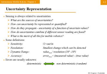
• Sensing is always related to uncertainties.
• What are the sources of uncertainties?
• How can uncertainty be represented or quantified?
• How do they propagate - uncertainty of a function
  of uncertain values?
• How do uncertainties combine if different sensor
  reading are fused?
• What is the merit of all this for mobile
  robotics?
• Some definitions
• Sensitivity Gout/in
• Resolution Smallest change which can be
  detected
• Dynamic Range valuemax/ resolution (104 -106)
• Accuracy errormax (measured value) -
  (true value)
• Errors are usually unknown
• deterministic non deterministic (random)

2
Uncertainty Representation (2)
4.2

• Statistical representation and independence of
  random variables on blackboard

3
Gaussian Distribution
4.2.1
0.4
-1
-2
1
2
4
The Error Propagation Law Motivation
4.2.2

• Imagine extracting a line based on point
  measurements with uncertainties.
• The model parameters ri (length of the
  perpendicular) and qi (its angle to the
  abscissa) describe a line uniquely.
• The question
• What is the uncertainty of the extracted line
  knowing the uncertainties of the measurement
  points that contribute to it ?

5
The Error Propagation Law
4.2.2

• Error propagation in a multiple-input
  multi-output system with n inputs and m outputs.

6
The Error Propagation Law
4.2.2

• One-dimensional case of a nonlinear error
  propagation problem
• It can be shown, that the output
  covariancematrix CY is given by the error
  propagation law
• where
• CX covariance matrix representing the input
  uncertainties
• CY covariance matrix representing the propagated
  uncertainties for the outputs.
• FX is the Jacobian matrix defined as
• which is the transposed of the gradient of f(X).

7
Feature Extraction - Scene Interpretation
4.3
scene
signal
feature
Environment
inter-
sensing
treatment
extraction
pretation

• A mobile robot must be able to determine its
  relationship to the environment by sensing and
  interpreting the measured signals.
• A wide variety of sensing technologies are
  available as we have seen in previous section.
• However, the main difficulty lies in interpreting
  these data, that is, in deciding what the sensor
  signals tell us about the environment.
• Choice of sensors (e.g. in-door, out-door, walls,
  free space )
• Choice of the environment model

8
Feature
4.3

• Features are distinctive elements or geometric
  primitives of the environment.
• They usually can be extracted from measurements
  and mathematically described.
• low-level features (geometric primitives) like
  lines, circles
• high-level features like edges, doors, tables or
  trash cans.
• In mobile robotics features help for
• localization and map building.

9
Environment Representation and Modeling Features
4.3

• Environment Representation
• Continuos Metric x,y,q
• Discrete Metric metric grid
• Discrete Topological topological grid
• Environment Modeling
• Raw sensor data, e.g. laser range data, grayscale
  images
• large volume of data, low distinctiveness
• makes use of all acquired information
• Low level features, e.g. line other geometric
  features
• medium volume of data, average distinctiveness
• filters out the useful information, still
  ambiguities
• High level features, e.g. doors, a car, the
  Eiffel tower
• low volume of data, high distinctiveness
• filters out the useful information, few/no
  ambiguities, not enough information

10
Environment Models Examples
4.3

• A Feature base Model B Occupancy Grid

11
Feature extraction base on range images
4.3.1

• Geometric primitives like line segments, circles,
  corners, edges
• Most other geometric primitives the parametric
  description of the features becomes already to
  complex and no closed form solutions exist.
• However, lines segments are very often sufficient
  to model the environment, especially for indoor
  applications.

12
Features Based on Range Data Line Extraction (1)
4.3.1

• Least Square
• Weighted Least Square

13
Features Based on Range Data Line Extraction (2)
4.3.1

• 17 measurement
• error (s) proportional to r2
• weighted least square

14
Propagation of uncertainty during line extraction
4.3.1

• ? (output
  covariance matrix)
• Jacobian

15
Segmentation for Line Extraction
4.3.1
16
Angular Histogram (range)
4.3.1
17
Extracting Other Geometric Features
4.3.1
18
Feature extraction
4.3.2
Scheme and tools in computer vision

• Recognition of features is, in general, a complex
  procedure requiring a variety of steps that
  successively transform the iconic data to
  recognition information.
• Handling unconstrained environments is still very
  challenging problem.

19
Visual Appearance-base Feature Extraction (Vision)
4.3.2
20
Feature Extraction (Vision) Tools
4.3.2

• Conditioning
• Suppresses noise
• Background normalization by suppressing
  uninteresting systematic or patterned variations
• Done by
• gray-scale modification (e.g. trasholding)
• (low pass) filtering
• Labeling
• Determination of the spatial arrangement of the
  events, i.e. searching for a structure
• Grouping
• Identification of the events by collecting
  together pixel participating in the same kind of
  event
• Extracting
• Compute a list of properties for each group
• Matching (see chapter 5)

21
Filtering and Edge Detection
4.3.2

• Gaussian Smoothing
• Removes high-frequency noise
• Convolution of intensity image I with G
• with
• Edges
• Locations where the brightness undergoes a sharp
  change,
• Differentiate one or two times the image
• Look for places where the magnitude of the
  derivative is large.
• Noise, thus first filtering/smoothing required
  before edge detection

22
Edge Detection
4.3.2

• Ultimate goal of edge detection
• an idealized line drawing.
• Edge contours in the image correspond to
  important scene contours.

23
Optimal Edge Detection Canny
4.3.2

• The processing steps
• Convolution of image with the Gaussian function G
• Finding maxima in the derivative
• Canny combines both in one operation

(a) A Gaussian function. (b) The first derivative
of a Gaussian function.
24
Optimal Edge Detection Canny 1D example
4.3.2

• (a) Intensity 1-D profile of an ideal step edge.
  
• (b) Intensity profile I(x) of a real edge.
• (c) Its derivative I(x).
• (d) The result of the convolution R(x) G Ä I,
  where G is the first derivative of a Gaussian
  function.

25
Optimal Edge Detection Canny
4.3.2

• 1-D edge detector can be defined with the
  following steps
• Convolute the image I with G to obtain R.
• Find the absolute value of R.
• Mark those peaks R that are above some
  predefined threshold T. The threshold is chosen
  to eliminate spurious peaks due to noise.
• 2D Two dimensional Gaussian function

26
Nonmaxima Suppression
4.3.2

• Output of an edge detector is usually a b/w image
  where the pixels with gradient magnitude above a
  predefined threshold are white and all the others
  are black
• Nonmaxima suppression generates contours
  described with only one pixel thinness

27
Optimal Edge Detection Canny Example
4.3.2

• Example of Canny edge detection
• After nonmaxima suppression

28
Gradient Edge Detectors
4.3.2

• Roberts
• Prewitt
• Sobel

29
Example
4.3.2

• Raw image
• Filtered (Sobel)
• Thresholding
• Nonmaxima suppression

30
Comparison of Edge Detection Methods
4.3.2

• Average time required to compute the edge figure
  of a 780 x 560 pixels image.
• The times required to compute an edge image are
  proportional with the accuracy of the resulting
  edge images

31
Dynamic Thresholding
4.3.2

• Changing illumination
• Constant threshold level in edge detection is not
  suitable
• Dynamically adapt the threshold level
• consider only the n pixels with the highest
  gradient magnitude for further calculation steps.

(a) Number of pixels with a specific gradient
magnitude in the image of Figure 1.2(b). (b)
Same as (a), but with logarithmic scale
32
Hough Transform Straight Edge Extraction
4.3.2

• All points p on a straight-line edge must satisfy
  yp m1 xp b1 .
• Each point (xp, yp) that is part of this line
  constraints the parameter m1 and b1.
• The Hough transform finds the line
  (line-parameters m, b) that get most votes from
  the edge pixels in the image.
• This is realized by four stepts
• Create a 2D array A m,b with axes that
  tessellate the values of m and b.
• Initialize the array A to zero.
• For each edge pixel (xp, yp) in the image, loop
  over all values of m and bif yp m1 xp b1
  then Am,b1
• Search cells in A with largest value. They
  correspond to extracted straight-line edge in the
  image.

33
Grouping, Clustering Assigning Features to
Features
4.3.2

• Connected Component Labeling

34
Floor Plane Extraction
4.3.2

• Vision based identification of traversable
• The processing steps
• As pre-processing, smooth If using a Gaussian
  smoothing operator
• Initialize a histogram array H with n intensity
  values for
• For every pixel (x,y) in If increment the
  histogram

35
Whole-Image Features
4.3.2

• OmniCam

36
Image Histograms
4.3.2

• The processing steps
• As pre-processing, smooth using a Gaussian
  smoothing operator
• Initialize with n levels
• For every pixel (x,y) in increment the
  histogram

37
Image Fingerprint Extraction
4.3.2

• Highly distinctive combination of simple features

38
Example
4.XX
Probabilistic Line Extraction from Noisy 1D Range
Data

• Suppose
• the segmentation problem has already been solved,
• regression equations for the model fit to the
  points have a closed-form solution which is the
  case when fitting straight lines.
• that the measurement uncertainties of the data
  points are known

39
Line Extraction
4.XX

• Estimating a line in the least squares sense. The
  model parameters (length of the perpendicular)
  and (its angle to the abscissa) describe
  uniquely a line.
• n measurement points in polar coordinates
• modeled as random variables
• Each point is independently affected by Gaussian
  noise in both coordinates.

40
Line Extraction
4.XX

• Task find the line
• This model minimizes the orthogonal distances di
  of a point to the line
• Let S be the (unweighted) sum of squared errors.

41
Line Extraction
4.XX

• The model parameters are now found by
  solving the nonlinear equation system
• Suppose each point a known variance
  modelling the uncertainty in radial and angular.
• variance is used to determine a weight for
  each single point, e.g.
• Then, equation (2.53) becomes

42
Line Extraction
4.XX

• It can be shown that the solution of (2.54) in
  the weighted least square sense is
• How the uncertainties of the measurements
  propagate through the system (eq. 2.57, 2.58)?

43
Line Extraction? Error Propagation Law
4.XX

• given the 2n x 2n input covariance matrix
• and the system relationships (2.57) and (2.58).
  Then by calculating the Jacobian
• we can instantly form the error propagation
  equation () yielding the sought CAR

44
Feature Extraction The Simplest Case Linear
Regression
4.XX
45
Feature Extraction Nonlinear Linear Regression
4.XX
46
Feature Extraction / Sensory Interpretation
4.XX

• A mobile robot must be able to determine its
  relationship to the environment by sensing and
  interpreting the measured signals.
• A wide variety of sensing technologies are
  available as we have seen in previous section.
• However, the main difficulty lies in interpreting
  these data, that is, in deciding what the sensor
  signals tell us about the environment.
• Choice of sensors (e.g. in-door, out-door, walls,
  free space )
• choice of the environment model