Lecture 4 - Monte Carlo improvements via variance reduction techniques: antithetic sampling

1
Lecture 4 - Monte Carlo improvements via
variance reduction techniques antithetic
sampling

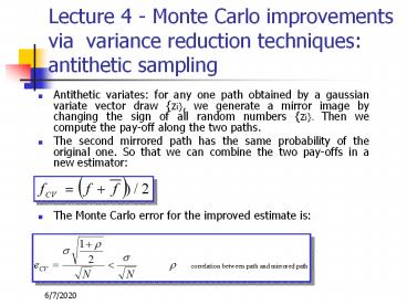
• Antithetic variates for any one path obtained by
  a gaussian variate vector draw zi, we generate
  a mirror image by changing the sign of all random
  numbers zi. Then we compute the pay-off along
  the two paths.
• The second mirrored path has the same probability
  of the original one. So that we can combine the
  two pay-offs in a new estimator
• The Monte Carlo error for the improved estimate
  is

2
Monte Carlo improvements via variance reduction
techniques control variates

• Control variates the Monte Carlo simulation is
  carried out both for the original problem as well
  as a similar problem for which we have a closed
  form solution. Being
• f the option value we want to estimate and
• y the analytical exact value of the auxiliary
  option
• an improved estimator of f is

• As a consequence of the above relations, control
  variates become more and more efficient as the
  auxiliary option is more correlated (or
  anti-correlated) with the original option, i.e.
  when the two problems are similar.

3
Monte Carlo improvements via variance reduction
techniques control variates and p

• Let us back to the problem of estimate p. A good
  choice for a control variable is a polygon with n
  edges inscribed in the circle. Indeed
• a closed formula exists for any value of n
• it has an high superposition with the circle

Stochastic term

• The error scales again as 1/sqrt(N) but with a
  smaller proportional constant

4
Monte Carlo improvements low discrepancy
sequences Quasi Monte Carlo

• In the standard Monte Carlo the error decreases
  slowly, as 1/sqrt(N), with number of samples, N,
  because draws do not fill in the space in a
  regular way. Indeed some gaps are present
  (clustering effects).
• In low discrepancy sequences the points are
  chosen in order to fill in the space more
  regularly and uniformly, without inhomogeneities.
  As a result the function to be integrated
  converges not as one over the square root of the
  number of samples (N) but much more closely as
  one over N (Quasi Monte Carlo).

5
Monte Carlo improvements low discrepancy
sequences definition and results

• The most famous algorithms to generate low
  discrepancy numbers are the Sobol and Halton
  sequences.
• The discrepancy is a measure of how inhomogeneous
  a set of D-dimensional vectors of random numbers
  fills in a unit hypercube.
• By definition, in a low discrepancy sequence (in
  D dimension), the discrepancy scales with the
  number of draws, N, as

6
Monte Carlo improvements low discrepancy
sequences high dimensional behavior

• Pros For a given precision, a lower number of
  scenarios are needed.

• Cons
• The convergence speed depends on problem
  dimension (making the method inefficient in very
  high dimensions).
• Quasi Monte carlo simulation are not reliable
  when high dimensions are involved, with a
  breakdown of homogeneity along some hyper-planes.

7
Monte Carlo pros and cons

• Pros
• Can be used in high dimensional problems.
• Easy to implement
• Easily extensible to any type of pay-off

• Cons
• Heavy from a computational point of view.

8
Conclusion

• We have presented a powerful numerical technique
  to price exotic options the Monte Carlo method.
• Numerical methods in finance will become more and
  more important due to the rapid growth in
  financial markets of the exotic products, with a
  clear trend to increase the complexity embedded
  in the exotic options.
• References P. Jackel - Monte Carlo Methods in
  Finance, Wiley Finance, (2002).