FT Representation of DT Signals:

1
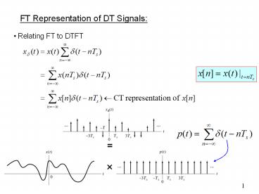
FT Representation of DT Signals

• Relating FT to DTFT

2
a) DTFT of xn
b) FT of CT signal
3

• Sampling. The figure shown 2 slides earlier

• Continuous-time representation of discrete-time
  signal xn

4
(No Transcript)
5
The FT of a sampled signal for different
sampling frequencies.Spectrum of continuous-time
signal.Spectrum of sampled signal when ?s
3W.Spectrum of sampled signal when ?s 2W. (d)
Spectrum of sampled signal when ?s 1.5W.
6

• Observations
• FT of a sampled signal x(jw) shifted by integer
  multiples of ws
• 2)

7
(No Transcript)
8
DTFT of sampled signal xn and FT of xd(t)
Example 4.9, p366
E
9
The effect of sampling a sinusoid at different
rates (Example 4.9). (a) Original signal and FT.
(b) Original signal, impulse sampled
representation and FT for Ts ¼. (c) Original
signal, impulse sampled representation and FT for
Ts 1. (d) Original signal, impulse sampled
representation and FT for Ts 3/2. A cosine of
frequency ?/3 is shown as the dashed line.
10
Problem 4.10, p368
E
Draw the FT of a sampled version of the CT signal
having the FT depicted By the following figure
for (a) Ts1/2 and (b) Ts2.
(a) Ts1/2, ws4p.
(b) Ts2, wsp.
11
(No Transcript)
12
Downsampling Let
E
13
(No Transcript)
14
(No Transcript)
15
Figure 4.29 (p. 372)Effect of subsampling on
the DTFT. (a) Original signal spectrum. (b) m
0 term, Xq(ej?), in Eq. (4.27) (c) m 1 term in
Eq. (4.27). (d m q 1 term in Eq. (4.27).
(e) Y(ej?), assuming that W lt ?/q. (f) Y(ej?),
assuming that W gt ?/q.
16
Sampling theorem
E
Example 4.12, p347
17
Ideal reconstruction

1. Spectrum of original signal.Spectrum of sampled
   signal.(c) Frequency response of reconstruction
   filter.

18
(No Transcript)
19
Figure 4.36 (p. 377)Ideal reconstruction in the
time domain.
20
Figure 4.37 (p. 377)Reconstruction via a
zero-order hold.

• Ideal reconstruction is not realizable
• Practical systems could use a zero-order hold
  block
• This distorts signal spectrum, and compensation
  is needed

21
Figure 4.38 (p. 378)Rectangular pulse used to
analyze zero-order hold reconstruction.
22
Figure 4.39 (p. 379)Effect of the zero-order
hold in the frequency domain.(a) Spectrum of
original continuous-time signal.(b) FT of
sampled signal.(c) Magnitude and phase of
Ho(j?).(d) Magnitude spectrum of signal
reconstructed using zero-order hold.
23
Figure 4.40 (p. 380)Frequency response of a
compensation filter used to eliminate some of the
distortion introduced by the zero-order hold.
Anti-imaging filter.
24
Figure 4.41 (p. 380)Block diagram of a
practical reconstruction system.
25
Figure 4.43 (p.383)Block diagram for
discrete-time processing of continuous-time
signals. (a) A basic system. (b) Equivalent
continuous-time system.
26
Idea find the CT system
0th-order S/H
27

• If no aliasing, the anti-imaging filter Hc(jw)
  eliminates frequency
• components above ws/2, leaving only k0 terms

• If anti-aliasing and anti-imaging filters are
  chosen to compensate
• the effects of sampling and reconstruction, then

28

• Oversampling
• Sampling rate must be greater than Nyquist rate
  to relax anti-aliasing filter design
• Let Ws be cutoff frequency of anti-aliasing
  filter Ha(jw) and W be the maximum frequency of
  desired signal
• Then, to avoid aliasing,

• Due to DSP, noise aliases are not of concern,
  thus

(see figure next slide)
29
Figure 4.44 (p. 385)Effect of oversampling on
anti-aliasing filter specifications. (a) Spectrum
of original signal. (b) Anti-aliasing filter
frequency response magnitude. (c) Spectrum of
signal at the anti-aliasing filter output. (d)
Spectrum of the anti-aliasing filter output after
sampling. The graph depicts the case of ?s gt 2Ws.
30

• Decimation (downsampling)
• To relax design of anti-aliasing filter and
  anti-imaging filters, we wish to use high
  sampling rates
• High-sampling rates lead to expensive digital
  processor
• Wish to have
• High rate for sampling/reconstruction
• Low rate for discrete-time processing
• This can be achieved using downsampling/upsamplin
  g

31
(No Transcript)
32
Figure 4.45 (p. 387)Effect of changing the
sampling rate. (a) Underlying continuous-time
signal FT. (b) DTFT of sampled data at sampling
interval Ts1. (c) DTFT of sampled data at
sampling interval Ts2.
33
Figure 4.46 (p. 387)The spectrum that results
from subsampling the DTFT X2(ej?) depicted in
Fig. 4.45 by a factor of q.
Figure 4.48 (p. 389)Symbol for decimation by a
factor of q (downsampling).
34
Figure 4.47 (p. 388)Frequency-domain
interpretation of decimation. (a) Block diagram
of decimation system. (b) Spectrum of
oversampled input signal. Noise is depicted as
the shaded portions of the spectrum. (c) Filter
frequency response. (d) Spectrum of filter
output. (e) Spectrum after subsampling.
35
Upsampling (zero padding)
36
Figure 4.49 (p. 390)Frequency-domain
interpretation of interpolation. (a) Spectrum of
original sequence. (b) Spectrum after inserting
q 1 zeros in between every value of the
original sequence.(c) Frequency response of a
filter for removing undesired replicates located
at ? 2?/q, ? 4?/q, , ? (q 1)2?/q. (d)
Spectrum of interpolated sequence.
37
Figure 4.50 (p. 390)(a) Block diagram of an
interpolation system.(b) Symbol denoting
interpolation by a factor of q.
38
Figure 4.51 (p. 391)Block diagram of a system
for discrete-time processing of continuous-time
signals including decimation and interpolation.
39

• FS representation of finite-duration nonperiodic
  signals
• Discrete-time periodic signals DTFS
  representation
• Continuous-time periodic signals FS
  representation
• For numerical computation, it is better to have
  BOTH discrete in time and discrete in frequency

40
Figure 4.52 (p. 392)The DTFS of a
finite-duration nonperiodic signal.
41
Figure 4.53 (p. 394)The DTFT and length-N DTFS
of a 32-point cosine. The dashed line denotes
X(ej?), while the stems represent NXk. (a)
N 32, (b) N 60, (c) N 120.
42
Figure 4.54 (p. 396)Block diagram depicting the
sequence of operations involved in approximating
the FT with the DTFS.
43
Figure 4.55 (p. 397)Effect of aliasing.
44
Figure 4.56 (p. 398)Magnitude response of
M-point window.
45
Figure 4.57 (p. 400)The DTFS approximation to
the FT of x(t) e-1/10 u(t)(cos(10t) cos(12t).
The solid line is the FT X(j?), and the stems
denote the DTFS approximation NTsYk. Both
X(j?) and NTsYk have even symmetry, so only
0 lt ? lt 20 is displayed. (a) M 100, N 4000.
(b) M 500, N 4000. (c) M 2500, N 4000.
(d) M 2500, N 16,0000 for 9 lt ? lt 13.
46
Figure 4.58 (p. 404)The DTFS approximation to
the FT of x(t) cos(2?(0.4)t) cos(2?(0.45)t).
The stems denote Yk, while the solid lines
denote (1/MY? (j?). The frequency axis is
displayed in units of Hz for convenience, and
only positive frequencies are illustrated. (a) M
40. (b) M 2000. Only the stems with nonzero
amplitude are depicted. (c) Behavior in the
vicinity of the sinusoidal frequencies for M
2000. (d) Behavior in the vicinity of the
sinusoidal frequencies for M 2010.
47
Figure 4.59 (p. 406)Block diagrams depicting
the decomposition of an inverse DTFS as a
combination of lower order inverse DTFSs. (a)
Eight-point inverse DTFS represented in terms of
two four-point inverse DTFSs. (b) four-point
inverse DTFS represented in terms of two-point
inverse DTFSs. (c) Two-point inverse DTFS.
48
Figure 4.60 (p. 407)Diagram of the FFT
algorithm for computing xn from Xk for N 8.