Traditional Approach to Requirements

1
LECTURE 6. Traditional Approach to Requirements
2
We discussed two key concepts of system
requirements modeling events and things. Now we
focus on what the system does when event occurs
activities and interactions. This lecture
presents the traditional structured approach to
activities and interactions.

• Differences Between Traditional and
  Object-Oriented Approaches Views of Activities
• Two approaches differ in the way the system is
  modeled and implemented.
• Traditional approach
• (using entity-relationship diagrams etc.)
  views a system as a collection of processes (like
  computer programs, a set of instructions that
  execute in sequence)
• When the process executes it interacts
  with data (reads data values and then writes data
  values back to the data file
• So traditional approach emphasizes
  processes, data, inputs/outputs
• Object Oriented approach (OO)
• (using class diagrams etc.) views a
  system as a collection of interacting objects
  which are capable of their own behavior (called
  methods) which allow the objects to interact
  with each other and with people using the system
• There are NO conventional processes and
  data files per se, just interacting objects
• Figure 6-1 summarizes the differences between two
  approaches.

3
FIGURE 6-1 Traditional versus OO approaches.
II. Data Flow Diagrams (DFD) Is the most
commonly used process model. Data Flow Diagram
(DFD) is a graphical system model that shows all
of the main requirements for an information
system in one diagram inputs, outputs,
processes and data storage Everyone working on
the project (and end users) can see all the
aspects of the project in the diagram with
minimal training (simple only 5 symbols)
Figure 6-2 presents DFD symbols.
4
FIGURE 6-2 Data flow diagram symbols.
5
Example of a Data Flow Diagram Figure 6-3
represents a portion of the RMO CSS
FIGURE 6-3 A DFD showing the process Look up
item availability (as a fragment of the RMO
case).
The square is an external agent (a person or
organization, outside the boundary of a system
that provides data inputs or accepts data
outputs) The rectangle with rounded corners is
a process (named Look up item available and can
be referred to by its number, 1) A process
defines rules (algorithms or procedures) for
transforming inputs into outputs The lines with
arrows are data flows (represents movement of
data). Figure 6-3 shows two data flows between
Customer and process 1 a process input Item
inquiry and process output named Item
availability details The flat three-sided
rectangle is a data store (a file or part of a
database that stores information about data
entity) Fig. 6-3 corresponds to event Customer
wants to check item available). DFD shows the
system activity in response to this event in
graphical form. But some piece of information on
the DFD is not in the event table the data
stores with information on items availability.
The DFD integrates processing triggering by
events with the data entities modeling by the ERD
(see Figure 6-4).
6
FIGURE 6-4 The DFD integrates the event table and
the ERD.
7

• Data Flow Diagrams and Levels of Abstraction
• DFD may reflect the processing at either a
  higher level (more general view of the system) or
  at lower level (a more detailed view of one
  process)
• These differing views of the system (higher
  level versus low level) creates the levels of
  abstraction
• DFD is a modeling technique that breaks the
  system into a hierarchical set of increasingly
  more detailed models
• Higher level processes in a DFD can be
  decomposed into separate lower level DFD (or some
  other diagram)
• Context Diagrams
• A context diagram is a DFD that summarizes all
  processing activity within the system in single
  process symbol
• Describes highest level view of a system
• All external agents and all data flows into and
  out of a system are shown in the diagram
• The whole system is represented as one process
• Example Figure 6-5 shows the context diagram
  for a university course registration system that
  interacts with 3 agents academic department,
  student, and faculty member

8
FIGURE 6-5 A context diagram for a course
registration system.
Academic department supplies information on
offered courses, students request enrollment in
offered courses, and faculty members receive
class list when the registration period is
complete.
9
Notes on Context Diagram Useful for showing
system boundaries (represents the system scope
within the single process plus external agents)
External agents that supply or receive data from
the system are outside the system scope Data
stores are not usually shown in the context
diagram since they are considered to be within
the system scope It is the highest level of
DFD Context diagram does not show any details
of what takes place within the system Figure 6-6
shows the context diagram for the RMOs CSS.
More then 30 data flows are shown Involves nine
different external agents The data flows come
from the event table they are triggers and
responses for all of the events
10
FIGURE 6-6 A context diagram for RMOs CSS.
11

• DFD Fragments
• DFD fragment is a DFD that represents the
  system response to one event within a single
  process symbol
• A fragment is created for each event in the
  event list it is a self-contained model showing
  how the system responds to a single event
• Created one at a time
• Figure 6-7 shows the three DFD fragments for a
  course registration system
• Each fragment represents all processing for an
  event within a single process symbols (shows
  details of interactions between the process,
  external agent and internal data store)
• The data stores in the DFD fragment represent
  entities in the ERD (each DFD fragment shows only
  those data stores that are actually needed to
  respond to the event)
• Figures 6-8 and 6-9 show the DFD fragments from
  the RMO case (there are 20 DFD fragments, the
  same number of events as in the RMO event table.

12
FIGURE 6-7 DFD fragments for the course
registration system.
13
FIGURE 6-8 DFD fragments for the RMOs CSS (part
1).
14
FIGURE 6-9 DFD fragments for the RMOs CSS (part
2).
15

• The Event-Partitioned System Model
• The entire set of DFD fragments can be combined
  on a single DFD called the event-partitioned
  system model or diagram 0
• Diagram 0 shows the entire system on a single
  DFD (in greater detail than on the context
  diagram)
• Figure 6-10 shows a set of four related DFDs
• The top diagram shows the Context diagram for
  course registration (same as fig. 6-5)
• The diagram below that is the event-partitioned
  model (i.e. diagram 0). It is a decomposition of
  the single process from the context diagram AND
  is a combined version of the three DFD fragments
  shown in Figure 6-7. Each process on diagram 0
  represents processing for a single event.
• The third DFD shows a single DFD fragment
  corresponding to process 1 on diagram 0 (since
  there are three processes on diagram 0, there
  should be three should be three separate DFD
  fragments, one for each process or event, but
  only one is shown)
• Finally, Diagram 1 is a decomposition of the
  process 1 in DFD fragment 1

16
FIGURE 6-10 Layers of DFD abstraction for the
course registration system.
17
Dividing the system into subsystems The RMO
customer support system involves 20 events,
therefore the event-partitioned system model
(diagram 0) would contain 20 processes
Such a diagram would be crowded and difficult to
read! A solution to this problem is to divide
the system into subsystems Events are grouped
into related subsystems based on similarities
in Interactions with external agents
Interactions with database stores Required
processing (in the RMO example, we can break up
the CSS into 4 subsystems (see Figure 6-11)
FIGURE 6-11 RMO subsystems and events for each
subsystem.
18
Next Step the subsystem DFD is created and
then decomposed into event-partitioned models
(one for each subsystem) Figure 6-13 shows the
RMO subsystem DFD (according to Figure 6-11).
Note several external agents (Shipping,
Customer, Management and Bank) are presented in
multiple places to minimize crossing data flows
and improve readability. By convention, a line is
drawn at a 45- degree angel in a corner of any
external agent symbol that appears multiple
times. Figure 6-14 shows event-partitioned view
of one of four subsystems Order-entry
subsystem (the event-partitioned DFDs for the
other three subsystems should also be created).
The model has 5 processes within it.
19
FIGURE 6-13 The RMO subsystem DFD.
20
FIGURE 6-13 The event-partitioned model of the
order-entry system.
21
Summary - Relationship of all these
diagrams Figure 6-12 shows the relationship
among DFD abstraction levels when subsystems are
defined
FIGURE 6-12 The relationship among DFD
abstraction levels when subsystems are defined.
22
The figure starts off with the context diagram
(entire system as one process), which breaks down
to the subsystem diagram (one process per
subsystem) The subsystem diagram is, in turn,
decomposed into a set of the event-partitioned
subsystem diagrams (There is no single diagram 0.
Instead, there is an event-partitioned DFD for
each of the subsystems. Each event-partitioned
DFD is a diagram 0 for a single
subsystem.) Decomposing Processes to see Details
of One Activity Sometimes certain DFD fragments
involve a lot of processing that the analyst
needs to explore in more detail. Using the same
principle of breaking down the model to more
detailed level, we can take a DFD fragment and
decompose it into subprocesses (just like the
context diagram is decomposed into diagram 0)
Such decomposition helps the analyst learn more
about the requirements while producing needed
documentation Figure 6-15 shows an example of
more detailed diagram for DFD fragment 2, Create
the new order. The diagram decomposes process 2
into 4 subprocesses Record customer
information, Record order, Record order
transaction and Produce confirmation Since
fragment Create new order was the second DFD
fragment defined for the RMO example (see fig.
6-8) we will label processes inside of it as
processes 2.1, 2.2, 2.3 and 2.4.
23
FIGURE 6-15 A detailed diagram for Create new
order (diagram 2).
24
The first step begins when the customer
provides the information making up the New
order data flow (it contains all of the
information about the customer and the items the
customer wants to order) Process 2-1 stores the
customer information in the data store Customer
(creating a new customer record or updating
existing customer information) and sends the rest
of the information about the order on to process
2.2 (a data flow Order details) Process 2-2
takes the Order details data flow and creates a
new order record by adding data to the Order
data store. For each item ordered, the stock on
hand and current price are looked up in the
Product item and Inventory item data store.
(If there is adequate stock on hand, an order
item record is created for that item, and the
stock on hand for the inventory item is changed.
This repeats until all items have been
processed) Process 2.2 adds up the total amount
due for the order (price times quantity for each
item) and sends the data flow Transaction
details to process 2.3 to record the transaction
(Transaction details include the order number,
amount and credit information) Process 2.3
should be a real-time link to a credit bureau to
get authorization for the customers credit card.
If the credit card is approved, a record of the
transaction is created in the Order transaction
data store, and a data flow for the transaction
goes directly to the bank The final process
produces the order confirmation for the customer
and the order details that go to shipping. Using
the order number, process 2-4 looks up data on
the order and produces the required outputs.
25
FIGURE 6- Incorrect and correct way to draw DFD.
26

• Physical and Logical DFDs
• A DFD can be a physical system model, a logical
  system model or a blend of the two
• If the DFD is a logical model then it leaves
  out low level physical details and assumes that
  the system will be implemented with a perfect
  technology, e.g. diagram in Figure 6-15 is a
  logical model, it does not present any technical
  details
• - What kind of computer is doing the
  processing (a desktop system, centralized
  mainframe system or networked client-server
  system, or could the entire process be carried
  out by people manually, without any computer at
  all)
• - Are data stores sequential computer files
  or tables in a relational database or files of
  papers in a file cabinet
• - How does the system gets the data flow New
  order from the customer by clicking check boxes
  and list boxes in a Windows application, or on a
  web page, or by manually filling out a form that
  a clerk types into the system, or by talking to
  the clerk over the phone
• If the DFD is a physical model then it includes
  details of the information technology (they are
  embedded in the model). Figure 6-16 is an example
  of a physical system model. The technology
  assumption is embedded in the name of process 1.1
  Making copies for department chairs it is a
  manual task, which implies that the data store
  Old schedule and the data flows into and out of
  process 1.1 are papers, etc.

27
FIGURE 6-16 A physical DFD for scheduling courses.
28
Physical DFDs are developed and used during the
last stages of analysis or early stages of
design. They are useful models for describing
alternative implementations of a system prior to
develop more detailed design models. Evaluating
DFD Quality A quality set of DFDs is
Readable Internally consistent
Accurately represents system requirements There
is a few simple rules to evaluate the quality of
DFDs. Minimizing complexity People have a limited
ability to manipulate complex information. If it
is too much, they experience a phenomenon called
information overload (i.e. difficulties with
information understanding) The key to avoiding
information overload is to divide information
into small and relatively independent subsets.
Each subset should contain an amount of
information that can be examined and understood
in isolation. A layered set of DFDs is an example
of dividing a large set of information into
small, independent subset There are two single
rules to avoid information overload - 7?2
- Interface minimization
29
The 7?2 rule (or Millers Number) derives from
psychology research. It shows that the number of
information chunks a person can remember and
manipulate at one time varies between five and
nine larger number of chunks causes
information overload (Information chunks may be
names, words in a list or components of a
picture). Applications of this rule to DFDs
construction include - No more than 7?2
processes should be presented on a single DFD
- No more than 7?2 data flows should enter or
leave each component of a DFD (i.e. a process,
data store, data element)  Interface
minimization is directly related to the 7?2 rule.
An interface is a connection to some other part
of a problem or description. The processes on a
DFD are related to other processes, entities and
data stores by data flows (i.e. they have
interface). A single process with a large number
of interfaces (data flows) may be too complex to
understand. The solution of this problem is to
divide the process into two or more processes,
each with a fewer amount of interfaces. Data
Flow Consistency To detect errors and omissions
in a set of DFDs, an analyst should first look
for three common and easily identifiable
consistency errors Differences in data flow
for a process and its decomposition Data
outflows without corresponding data inflows
Data inflows without corresponding outflows
30
A process decomposition shows the internal
details of a higher-level process in a more
detailed form. The data content of flows to and
from a process at one DFD level should be
equivalent to the content of flows to and from
all process decomposition. This equivalency is
called balancing, and the higher-level DFD and
the process decomposition DFD are said to be in
balance. Another type of DFD inconsistency
is called a black hole, i.e. a process with a
data input that is never used to produce a data
input. The following rules help to avoid the
black holes -         - All data that flow into
a process must flow out of the process or be used
to generated data that flow out of the
process -         - All data that flow out of a
process must have flowed into the process or have
been generated from data that flowed into the
process Figure 6-17 is an example where
the first rule is violated. Data elements A, B,
and C flow into the process but do not flow out.
Data element A is used in calculations within the
process and is a necessary input. Data elements B
and C play no role in generating process output
and should be eliminated as unnecessary
inflows.
31
FIGURE 6-17 A process with unnecessary data input
(a black hole).
Figure 6-18 is an example where the second rule
is violated. Data elements A, B and Y flow out of
the process. Data element Y is computed by an
algorithm based on data element A. However, data
element B does not flow into the process and is
not computed by internal processing logic. Thus,
data element B indicates either an error in the
data flow outputs (B should be eliminated) or an
omission in the internal processing logic (the
rule that determine B is missing). A data element
such as B is called a miracle, i.e. a process
with a data output that is created out of nothing
( miraculously appears)
32
FIGURE 6-18 A process with an impossible data
output (a miracle).
Black hole and miracle problems apply to both
processes and data stores Most CASE tools
automatically perform data flow consistency
checking   III. Documenting DFD Components In the
traditional approach, DFDs show three type of
internal system component processes, data flows
and data stores. The details of each component
need to be described.
33
Process Descriptions Each process on a DFD must
be formally defined There are several options
for process definition including decomposition.
In a process of decomposition, a higher-level
process is formally defined by a DFD that
contains lover-level processes, which, in turn,
may be further decomposed into even lower-level
DFDs. Eventually a point will be reached when a
process becomes so simple that it can adequately
be described by another process description
method, i.e. without next lower-level DFD.
These description methods include -
Structured English - Decision tables -
Decision trees These models describe the
process as an algorithm. Structured English
Uses brief statements in form of instructions,
repetition of instructions and if-then-else logic
to write process specifications (Figure 6-19 is a
structured English example) It looks like
programming statement but this is not necessarily
a computer program (its a combination of
structured programming with narrative
English) Figure 6-20 shows a process description
for RMOs CSS.  
34
FIGURE 6-19 A structured English example.
FIGURE 6-20 RMO process 2.1 Record customer
informationand its structured English
description.
35
Limitations of structured English Good
for representing processes with (1) many
sequential processing steps, and (2)
relatively simple control logic Not so good
for showing     (1) complex decision logic
(see Figure 6-21) and   (2) if there
are few or no sequential processing
steps
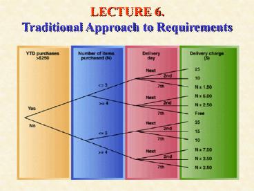
FIGURE 6-21 A structured English process
description for determining delivery charges.
36
Decision Table and Decision Tree can summarize
complex decision logic better than structured
English Decision Table is a tabular
representation of processing logic containing
decision variables, decision variable values and
actions or formulas Decision Tree is a
graphical description of process logic that uses
lines organized like branches of a tree Figures
6-22 and 6-23 show a decision table and decision
tree representing the same logic as the
structured English example in Figure 6-21
FIGURE 6-22 A decision table for calculating
shipping charges.
Both make the descriptions more readable than
structured English the decision table is more
compact, but decision tree is easier to read
37
FIGURE 6-23 A decision tree for calculating
shipping charges.
38
Making a Decision Table (Figure 6-22) Step 1
Identify the decision variables and their
possible values (value ranges) -Year to date
purchases (YTD) has two ranges less than 250
and greater or equal to 250 - Number of items
ordered has two relevant ranges less than or
equal to three and greater than or equal to four
- Delivery date has tree possible values
next day, second day and seventh day Step 2
Compute the number of decision variable
combinations as the product of their possible
values - In our case, there are 2x2x3 12
combinations Step 3 Construct a table with the
number of columns equal to the number of decision
variable combinations plus one (for decision
variables names) and with rows for each decision
variable plus for each process action or
computation - In our case there are 12 1
13 columns and four rows in the table Step 4
Put variable with fewest possible value ranges in
the first row of the table - In this example
we could put either YTD or number of items, we
chose YTD purchases. Table so far is just one
row YTD Purchases gt 250
YES
NO Step 5 put variable with next fewest
possible value ranges as next row in the table,
to now get YTD Purchases gt
250 YES
NO Number of
Items (N) N lt 3 N gt 4
N lt 3 N gt 4
39

• Step 6 Continue inserting rows as in step 5
  until all decision variables are included in the
  table. Table now looks like
• YTD Purchases gt 250 YES
  NO
• Number of Items (N) N lt3
  Ngt4 Nlt3 Ngt4
• Delivery Day Next 2nd
  7th Next 2nd 7th Next 2nd 7th Next
  2nd 7th
• Step 7 Add a row for each calculation or
  action.
• - In our case, the row contains a value or
  formula to determine shipping charge (e.g.
  shipping is free for customers with YTD purchases
  greater than 250, ordering more than three items
  and seventh-day delivery).
• Finally, we have the complete table as in Figure
  6-22.
• Making a Decision Tree
• Decision tree can be constructed in almost the
  same way as a decision table (only difference is
  that rows in a decision table are columns of a
  decision tree just flip the table sideways and
  you get the tree as in Figure 6-23)
• Sometimes an analyst might use all 3 ways
• Structured English
• Decision Table
• Decision Tree

40
There may be several actions associated with a
set of conditions in a Decision Table Figure 6-24
shows a table where if the customer is new and if
an item is on backorder for gt 25 days then two
things are done (a) include detailed
return instructions (b) expedite delivery
FIGURE 6-24 A decision table with multiple action
rows.
Data Flow Definitions Data flow is a
collection of data elements Data flow
definition is a textual description of a data
flows content and internal structure. It lists
all the elements, e.g. a New Order data flow
consists of Customer Name, Customer-Address,
Credit-Card-Information, Item-Number and Quantity
41
There are two approaches to data flow
definitions One approach is simply to list the
data elements (Figure 6-25) Algebraic notation
can be used (Figure 6-26) the data flow equals
to or consists of one element plus another one,
etc groups of elements that can have many values
are enclosed in curly braces (In this case, New
Order equals to the customer name plus
credit card information plus one or more
inventory items number and quantity.  
FIGURE 6-25 Data flow definitions simply listing
elements.
FIGURE 6-26 Algebraic notion for data flow (New
Order).
Figures 6-27 and 6-28 show a complex report and
its corresponding data flow definition (the
structure of the report is a repeating group over
products with an embedded repeating group over
inventory items).
42
FIGURE 6-27 A sample report produced by the RMOs
CSS.
43
FIGURE 6-28 A data flow definition for the RMOs
products and items report.
44
Data Element Definitions Data Element
Definitions describe a data type (e.g. string,
integer, floating point, or Boolean)
Lengths are usually defined for strings
Numeric values usually have a minimum and maximum
value (a valid range) Might define special
codes (e.g. code A means ship immediately, code B
hold for one day and code C hold shipment
pending confirmation) Figure 6-29 is a sample of
data element definitions.  
FIGURE 6-29 Data element definition.
45
Data Store Definitions A data store on the DFD
represents a data entity on the ERD (so, no
separate definition is needed, just a note
referring to the ERD for details) If a data
store are not linked to an ERD, a definition is
provided as a collection of elements (like did
for data flows) DFD Summary Four components of
a traditional analysis model are Data flow
diagrams Entity-relationship diagram
Process definitions Data definitions They
form an interlocking set of specifications for
system requirements DFD shows highest-level
view of the system Other components describe
some aspect of DFD These models were created in
the 1970s and 1980s as a part of the structured
analysis methodology IV. Information
Engineering Models (we are not covering)
46
V. Representing Locations and Communications
Some kind of physical issues is needed at early
stages of design   Number of locations of
users Processing and data access
requirements of users at specific locations
Volume and timing of processing and data access
requests This information is required to make
initial design decisions (e.g. the distribution
of computer systems, application software and
database components, determining network capacity
among users and processing locations) The first
step in gathering such information is
identification and describing the locations where
work is being or will be performed and presenting
them in graphical form of a location diagram
Location diagram is a diagram or map that
identifies all of the processing locations of a
system (business offices, warehouses,
manufacturing facilities). Figure 6-35 is an
example of location diagram for RMO
47
FIGURE 6-35 The RMO location diagram.
48
The next step is to list the functions that are
performed by users at each location in form of
activity-location matrix (a table that describes
the relationship between processes and the
locations where they are performed). Each row is
a system activity, each column is a location.
Figure 6-36 shows activity-location matrix for
the RMO. Other matrix can be created to
highlight access requirements, which lists
activities and data entities in an activity-data
matrix. Activity-data matrix is a table that
describes stored data entities, the locations
from which they are accessed and the nature of
the access (i.e. which activities require access
to the data). Source of this information is
- the DFD fragments (traditional approach) and
- sequence diagrams (OO approach). Figure 6-37
shows an activity-data matrix for the RMO (in the
cells of the matrix, additional information is
shown to clarify what the activity does to the
data C means the activity creates new data, R
means it reads data, U means the activity updates
data and D means it delete data). The acronym
CRUD is often used to describe this type of
matrix.
49
FIGURE 6-36 Activity-location matrix for the
RMOs CSS.
50
FIGURE 6-37 Activity-data matrix for the RMO.
51
VI. Workflow Modeling A workflow is the flow of
control through a processing activity as it moves
among people, organizations, computer programs,
and specific processing steps (i.e. it is the
sequence of processing steps that completely
handles one business transaction or customer
request) It encompasses Trigger
The processing steps that respond to a trigger
Participants (or actors) can be people and
machines Flow of data Workflow models can
be developed and checked with users to gain
better understanding of a system or
organization Can also be developed during the
transition between analysis and structured
design Can be used to describe complex
interactions among system components and
participants Can be used to describe
alternative approaches to system organization and
human-computing interaction Also used when
performing business process reengineering (see
Lecture 4) No single method is used to model
workflows (usually include flow charts, data flow
diagrams and activity diagrams
52
DFD are good at capturing the flow of data
within a workflow but arent designed to
represent control flows Flow charts and
activity charts are specially designed to
represent control flow among processing steps,
but they dont represent data flow Figure 3-38
shows a workflow model for a university
scheduling process (An activity diagram is used
to represent the workflow rounded rectangles
represent processing steps, arrows represent
control flows, diamonds represent decisions and
horizontal bars represent synchronization points.
The model shows each processing step within a
vertical box that represents participant, i.e.
shows not only the flow of control among
processing steps but also among
participants). Figure 3-39 shows the workflow
model for the RMO telephone order entry process
(this model shows the interactions between the
customer, an order clerk and the automated
system).  
53
FIGURE 6-38 A workflow model of a university
scheduling system.
54
FIGURE 6-39 A workflow model for the RMO
telephone order entry system.
55
Readings
Todays lecture Chapter 6 The Traditional
Approach to Requirements For next lecture
Chapter 7 The Object-Oriented Approach to
Requirements