
Routing PowerPoint PPT Presentation
1 / 35
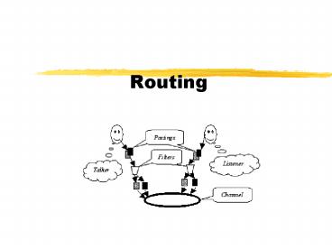
Title: Routing
1
Routing
2
Routing through switched networks
- Routing is the process of directing data to the
correct destination. - How difficult it is to route data depends on the
topology of the network. - Broadcast networks such as the bus and ring
topologies have no need of routing strategies. - The star topology only needs a central switching
hub to route data. - A tree topology passes data up the tree until it
reaches a common node with the destination. The
data is then passed down the appropriate branch.
There is a clear deterministic routing algorithm
that can be used. - A large mesh topology must employ sophisticated
routing techniques. There is no deterministic
approach to routing that will work on all mesh
topologies.
3
Routing Strategies
- There are two general approaches to routing
- Shortest Path Routing endeavours to set up the
routing tables so that data always travels along
a least cost path for any given
source-destination pair. - The cost of the path is defined as a linear sum
of the cost of each hop in the path. The cost
could be a fixed or variable quantity relating to
bandwidth, propagation delay, estimated
congestion, security or any combination of these. - Bifurcated Routing attempts to load all the links
equally. The idea is that this will spread the
load so that congestion does not occur in busy
regions of the network. - This generally leads to multiple routings for
data travelling between any given
source-destination pair.
4
Source Routing
- In source routing the sending host decides on the
path that the data will follow. - The host puts description of the route in the
packet or frame. - Of course, this implies that the host is aware of
the available routes. - Source routing is traditionally used in
interconnected token ring LANs. - If host A wants to transmit a frame to host C, it
must describe the route the frame must follow.
5
Source Routing
- When source routing is being used, the group bit
in the source address field is set to 1 (0 would
indicate that the frame is destine for another
host on the same LAN). - A list of 16-bit route designators follows the
source address field. Each designator consists
of a segment number and a bridge number. - Each segment is given a unique 12 bit code and
each bridge is given a 4-bit code (unique in each
LAN). - In our example, the route would look like
S1,B1,S2,B3,S4.The last 4 bits of the last
designator are ignored.
6
Source Routing
- Each bridge looks out for frames being routed
over it. - It does this by looking out for a segment ID code
followed by its own bridge number. - It stores the frame and waits for the opportunity
to transmit it over the next LAN segment. - If the destination host wants to send back a
reply, it only has to reverse the route
information. - In order to discover the route to a new host, the
source host must transmit discovery frames to all
LAN segments. - Each time a discovery frame passes through a
bridge, a new route designator is added to it. - The first discovery frame to reach the new host
will have discovered the fastest route (which is
transmitted back).
7
Source Routing
- Discovery frames are very good at finding the
fastest routes on relatively small groups of
interconnected LAN segments. - On very large networks, so many discovery frames
will be generated that they may flood the network
and cause congestion. - If a bridge or a LAN segment fails, a new
discovery frame must be issued to discover an
alternative route. - The host must store all the routes to all the
destinations it regularly sends data to. Storing
all this information can be cumbersome and adds
to the complexity of the communications software.
8
Transparent Routing
- Transparent routing is the opposite of source
routing. It is not the responsibility of the
host to supply the route but rather the network
to determine the route. - We have already seen an example of transparent
routing. The spanning tree algorithm is used to
map a tree topology onto a mesh topology in order
to determine routes for data. - The spanning tree algorithm is not suitable for
large mesh topologies since the node at the top
of the tree will become a communications
bottleneck. - Also large networks are subject to frequent
localised alterations. The spanning tree would
quickly become out of date and the spanning tree
algorithm would have to be run again.
9
Static Routing Tables
- An alternative way of transparently routing data
through a switched network is to use static
routing tables. - Each node in the network stores and forwards the
data. - Each node contains a routing table that lists the
best way to send data so that it gets to its
destination node. - The table will usually include an alternative
route so that any failures in the network can be
bypassed.
Unexpectedly, the node 1 to node 3 connection has
failed. The alternative is to send the data to
node 2. From node 2, the data gets sent to node 3
and then to node 5.
Device A is sending data to the device connected
to node 5 (address A5).
10
Static Routing Tables
- Packets of data enter the network with the
destination node address set as one of its
fields. - Each node examines this address field and looks
up the next node in its routing table. - If the node is unable to forward the packet to
the next appropriate node, it sends it to the
alternative node. - The contents of the routing tables are decided
when the network is set up. The table entries
are usually entered by network administrators. - The routing table contents should take account of
the networks topology and the most likely areas
for congestion in the network. - The tables can be adjusted locally to take
account of local alteration to the network.
11
Adaptive Routing
- Static routing tables may give good performance
under some conditions but not all. - The best routing tables for normal usage may be
the worst routing tables when the network gets
busy. - What we need are routing tables that adjust to
cope with changing conditions. - This is called adaptive routing.
- In adaptive routing, the nodes must measure the
performance of the local network. - With this information, the nodes can decide how
best to route data. - The sort of things measured include propagation
delay, throughput, error rates, etc.
12
Isolated Adaptive Routing
- Getting feedback from the network around a node
results in additional complexity and overheads. - An alternative is to allow each node to take
decisions based only on the information
immediately available to it. - This is called isolated adaptive routing.
- The information available to a node typically
consists of - A pre-loaded static routing table
- The current state of on-going connections (i.e.
free or busy) - The queue lengths of packets waiting to use each
route - The isolated adaptive routing algorithm is
programmed to make a choice between alternative
routes for sending packets.
13
Isolate Adaptive Routing
- Consider a node that has two routes available to
it. - There is a preferred high speed primary route
(weighted 3) and a lower speed secondary route
(weighted 1). - When a new packet arrives, the probability of it
going into a queues is proportional to the weight
plus the number of empty spaces available on the
queue (44 above). - If one queue is full, then the packet is placed
on the alternative queue. If both are full, the
packet is discarded.
14
Distributed Adaptive Routing
- A different adaptive routing algorithm was used
in ARPANET (the precursor of the Internet). - The object was to find paths of least transit
delay for network traffic. - The average delay for every link attached to a
node was measured every 10 seconds. This
information was then propagated to other nodes in
the system. - This allowed nodes to build up a dynamic database
of the fastest routes in the local network. This
information was then used to decide the best way
to route packets to their destination.
15
Distributed Adaptive Routing
- The overheads of the the ARPANET approach can be
considerable. - Packets are used to convey the delay information,
which themselves can introduce delays. - The earliest versions of ARPANET sent updated
information every 0.67 seconds. - Up to 50 of the network traffic was accounted
for by the delay information packets being
propagated. - By increasing the update interval time to 10
seconds and only sending updates when significant
changes occurred, the overheads were dramatically
reduced.
16
Flooding
- It is possible to dispense with a formal
systematic algorithm for routing. - Flooding is a method that has some applications
in military networks. - Copies of every packet are forwarded on every
outbound link except the one on which the packet
arrived. - Since a copy of the packet is sent over every
path in the network, a copy of the packet will
reach its destination in the shortest time
possible. - It has high resilience. Unless all paths are
severed, a copy of the packet will eventually
reach its destination. - Flooding is very wasteful of network capacity.
Multiple copies of the same packet use up most of
the capacity.
17
Routing with Bridges
18
Routing with Bridges
- There are three main techniques
- Fixed routing
- Spanning Trees
- Source routing
19
Fixed Routing
- Fixed route for every source-destination pair of
LANs. - Does not automatically respond to changes in
load/topology. - Statically configured routing matrix (pre-loaded
into bridge). - If alternate routes, pick shortest one.
- Rij first bridge on the route from i to j.
20
Fixed Routing Example
1
2
3
Source LAN
A B C D E
F G
LAN A
107
101
103
105
106
A
102
102
101
106
B
101
102
103
104
105
LAN B
LAN C
105
C
102
101
103
107
106
107
104
D
101
103
102
105
106
106
103
105
104
E
LAN D
107
102
103
E
F
G
104
105
106
105
107
106
102
101
F
103
4
5
6
7
102
101
106
107
105
103
G
Ex E-gt F 107 102 105.
21
Fixed Routing
- Each bridge keeps column for each LAN it
attaches. - Table From X derived from column x.
- Every entry that has the number of the bridge
results in entry.
101
From A
From B
Dest
Next
A A C A D - E - F
A G A
B
B
C
D B
E
F
G
- Problems..
- Simple and minimal processing.
- Too limited for networks with dynamically
changing topology.
22
Spanning Tree Routing
- Also known as transparent bridges.
- Bridge routing table is automatically maintained
(set up and updated as topology changes). - 3 mechanisms
- Address learning.
- Frame forwarding.
- Loop resolution.
23
Address Learning
- Problem determine where destinations are.
- Bridges operate in promiscuous mode, i.e., accept
all frames. - Basic idea look at source address of received
frame to learn where that station is (which
direction frame came from). - Build routing table so that if frame comes from A
on interface N, save A, N. When bridges first
start, all tables are empty. - So they flood every frame for unknown
destination, is forwarded on all interfaces
except the one it came from. - With time, bridges learn where destinations are,
and no longer need to flood for known
destinations.
24
Backward Learning
- Bridges look at frames (MAC) source address to
find which machine is accessible on which LAN.
LAN 4
A
C
B
LAN 1
B2
LAN 2
B1
LAN 3
If B1 sees frame from C on LAN 2, RT entry (C,
LAN2). Any frame to C on LAN1 will be
forwarded. But, frame to C on LAN2 will not be
forwarded.
25
Address Learning continued
- RT entries have a time-to-live (TTL).
- RT entries refreshed when frames from source
already in the table arrive. - Periodically, process running on bridge scans RT
and purges stale entries, i.e., entries older
than TTL. - Forwarding to unknown destinations reverts to
flooding.
26
Frame Forwarding
- Depends on source and destination LANs.
- If destination LAN (where frame is going to)
source LAN (where frame is coming from), discard
frame. - If destination LAN ! source LAN, forward frame.
- If destination LAN unknown, flood frame.
- Special purpose hardware used to perform RT
lookup and update in few microseconds.
27
Loop Problems
Loop Resolution Done by removing extra paths
by removing extra bridges.
B
LAN 1
B1
B2
LAN 2
A
1. Station A sends frame to B bridges B1 and B2
dont know B. 2. B1 copies frame onto LAN1 B2
does the same. 3. B2 sees B1s frame to unknown
destination and copies it onto LAN 2. 4. B1 sees
B2s frame and does the same. 5. This can go on
forever.
28
Definitions
- Bridge ID unique number (e.g., MAC address
integer) assigned to each bridge. - Root bridge with smallest ID.
- Cost associated with each interface specifies
cost of transmitting frame through that
interface. - Root port interface to minimum-cost path to
root. - Root path cost cost of path to root bridge.
- Designated bridge on any LAN, bridge closest to
root, i.e., the one with minimum root path cost.
29
Spanning Tree Algorithm
- 1. Determine root bridge.
- 2. Determine root port on all bridges.
- 3. Determine designated bridges.
- Initially all bridges assume they are the root
and broadcast message with its ID, root path
cost. - Eventually, lowest-ID bridge will be known to
everyone and will become root. - Root bridge periodically broadcasts its the
root. - Directly connected bridges update their cost to
root and broadcast message on other LANs they are
attached. - This is propagated throughout network.
- On any (non-directly connected) LAN, bridge
closest to root becomes designated bridge.
30
Source Routing
- Route determined a priori by sender.
- Route included in the frame header as sequence of
LAN and bridge identifiers. - When bridge receives frame
- Forward frame if bridge is on the route.
- Discard frame otherwise.
- No need to maintain routing table.
- Frame has all needed routing information.
- However, stations need to find route to
destination.
31
Route Discovery
- Finding all routes.
- If destination is unknown, source sends broadcast
route discovery frame. - Frame reaches every LAN.
- When reply comes back, intermediate bridges
record their id. - Source gets complete route information.
- Problem frame explosion.
- Route Selection
- Select minimum-cost route, e.g., minimum-hop
route. - If tie, choose the one that arrived first.
- Routes are cached with a TTL when TTL expires,
re-discover route.
32
Routers
- Operate at the network layer, i.e., inspect the
network-layer header. - Usually main router functionality implemented in
software. - Store-and-forward.
- Ability to interconnect heterogeneous networks
address translation, link speed and packet size
mismatch. - Router Goals
- Get data from source to destination. This may
require traversing many hops and involving
intermediate routers. - In contrast with data link layer frames from one
end of a wire to the other. - Network layer as lowest end-to-end transmission
layer multiple hops.
33
Routing and Internetworking
- Based on knowledge of network topology, choose
appropriate paths from source to destination. - Load balancing across routers and links.
- Avoid congestion.
- Network interconnection internetworking.
- Source and destination in different networks.
- For VCs, routers keep a table with (VC number,
outgoing interface) entries. - Packets only need to carry VC number.
- For datagrams, routing table.
- (destination, outgoing interface) entries.
- Each packet must carry destination address.
34
Routing Algorithms Metrics
- Routing is main function of network layer.
- Routing algorithm decides which route a packet
should take from source to destination. - For router which interface a packet should be
forwarded. - If datagram network, decision is made for every
packet. - If VC, decision is made only once when VC is
setup. - Routing algorithms can use different metrics when
building/selecting routes. - E.g.
- Number of hops.
- Delay.
- Bandwidth.
35
Adaptive Non-adaptive Routing
- Non-adaptive routing
- Fixed routing, static routing.
- Do not take current state of the network (e.g.,
load, topology). - Routes are computed in advance, off-line, and
downloaded to routers when booted. - Adaptive routing
- Routes change dynamically as function of current
state of network. - Algorithms vary on how they get routing
information, metrics used, and when they change
routes. - If router J is on optimal path between I and K,
then the optimal path from J to K also falls
along the same route. - Proof by contradiction.
Recommended
