Control System Analysis Cycle

1
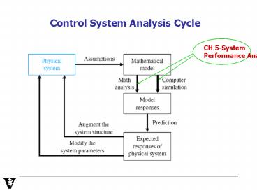
Control System Analysis Cycle
CH 5-System Performance Analysis
2
CH. 5 Performance of Feedback Control Systems

• This chapter describes how the input and the
  poles and zeros of the system will affect system
  performance, i.e. system output (or response).

3
CH. 5 Performance of Feedback Control Systems

• This chapter describes how the input and the
  poles and zeros of the system will affect system
  performance, i.e. system output or response.
• Topics to be covered
• - Input Signals for testing performance (5.2)
• - Performance of 1st-order Systems
• - Performance of 2nd-order Systems (5.3)
• - Root Location and the Transient Response
  (5.5)
• - Steady-State Error of Feedback Systems (5.6)
• - Design Example (5.9)
• - Performance Analysis using Matlab and
  Simulink
• (5.10,5.11)

4
System Performance

• System Responses
• 1. Time (or Transient) Response lt
• 2. Frequency (or Steady-State) Response (Ch.
  8)
• Key Concepts
• 1. System Characteristic Equation
• 2. Poles and Zeros

5
Impulse Response A Special Case of Time Response

• The impulse response is the response for control
  systems to an input d(t) where
• d(t) 1 (Table 2.3, p. 51).
• So, if the input is the impulse, the output
• is the inverse Laplace transform of the
  transfer function G(S)
• R(s)1 Y(s)G(S)
• or
  y(t)g(t)

G(s)
6
Matlab Command for Impulse Response impulse(sys)

• So, if the input is the impulse, the output is
  the inverse
• Laplace transform of the transfer function
  G(S)
• R(s)1
  Y(s)G(S)
• Matlab command for the unit impulse response of
  LTI systems is
• gtgtimpulse(sys) Plots the impulse response of
  an arbitrary LTI model sys. This model can be
  SISO or MIMO, i.e. state models. Zero initial
  state is assumed for state models.

G(s)
7
Example

• So, if the input is the impulse, the output is
  the inverse
• Laplace transform of the transfer function
  G(S)
• R(s)1
  Y(s)G(S)
• Ex. G(s)1/(sst) gt g(t)e-st, tgt0.

G(s)
8
Time (Transient) Response

• Let the system transfer function be
• G(s)p(s)/q(s). Eq.(2.45), p. 58
• Then,
• 1. The (System) Characteristic Eqn. is q(s)0.
• 2. Poles are the roots of q(s)o.
• 3. Zeros are the roots of p(s)0.

9
Example

• Consider the transfer function
• G(s)p(s)/q(s)(2s1)/(s23s2)
• gt
• Poles q(s) s23s20 gt s-1,-2
• Zeros p(s)2s10 gt s-1/2

10
Poles and System Stability

• Location of Poles will determine the system
  stability (Ch. 6)

11
Finding system poles and zeros

• Example pole and zero (Ch. 2, p. 107)

12
Commonly Used Input Signals(Table 5.1, Fig. 5.2,
p. 279)

• (a) Step (b) Ramp
  (c) Parabolic

r(t)A, tgt0
r(t)At, tgt0
r(t)At2, tgt0
13
Performance of First-Order Systems

• Ex. Transfer function of the RC circuit below
• (p. 53, Ch. 2)
• V1(s)(R1/Cs)I(s) and
• V2(s)I(s)(1/Cs)
• ? G(s)V2(s)/V1(s)1/(RCs1)
• where RC is called the time constant ?.

14
Transfer Function of First-Order Systems

• Ex. G(s)V2(s)/V1(s)1/(RCs1) where RC is called
  
• the time constant ?.
• ?In general,
• G(s) K/(?s1), where Ksystem DC gain
• (i.e.,
  KG(0)).
• R(s)
  Y(s)

G(s)
15
Performance of First-Order Systems

• G(s) K/(?s1), where Ksystem DC gain (G(0)),
• and ? time
  constant
• Step response R(s)1/s Y(s)
• gt
• Y(s)K/s K/(s1/?)
• gt
• y(t) K(1-e t/? )

G(s)
?
16
Performance of First-Order Systems

• G(s) K/(? s1), where Ksystem DC gain (i.e.,
  KG(0)).
• 1. Step response U(s)1/s gt
• Y(s)K/s K/(s1/? gt y(t)
  K(1-e -t/? )
• 2. Ramp response R(s)1/s2 gt
• Y(s) K/s2 K? /s K? /(s1/?)
• gt
• y(t) Kt - K? K? e t/?

ess Steady-state error
17
Transfer Function of a Second-Order Linear System

• Ex. A spring-mass-damper system
• From Ch. 2, Md2y/dt2bdy/dtkyu(t)
• gt
• G(s) 1/(Ms2 bs k)

18
Transfer Function of a 2nd-Order System

• Standard Form
• Y(s)G(s)/(1G(s))U(s)
• ?n2/(s22? ?ns ?n2)R(s) (5.7)
• where,
• ? (zeta)damping ratio
• ?nnatural frequency

19
Transfer Function of a 2nd-Order System

• Standard Form
• Y(s)G(s)/(1G(s))U(s)?n2/(s22? ?ns
  ?n2)R(s) (5.7)
• where,
• ? (zeta)damping ratio , ?nnatural
  frequency
• Notes Damping ratio is a real number between 0
  and 1, and defines the damping properties of the
  system, i.e.
• the smaller ? is, the bigger system
  oscillation becomes.
• Natural frequency or natural mode of a system
  determines system frequency response with no
  forcing function, i.e. u(t)0.

20
Fig. 5.5 Step Response of y(t) 1 (1/ß)e - ?
?nt sin(?n ß t ?)
? 0.1 0.2 0.7 1.0 2.0
21
Performance of a 2nd-Order System

• Unit Step Responce
• Y(s)G(s)R(s), R(s)1/s
• ?n2/s(s22? ?ns ?n2) (5.8)
• gt
• y(t) 1 (1/ß)e - ? ?nt sin(?n ß t ?)
  (5.9)
• where
• ß ?2

22
Ex. Effect of ?n on the step response (Figure
5.10)
23
Step Response of a 2nd-Order System

• Standard form G(s) ?n2/s(s2? ?ns ?n2)
• For complex poles, the unit step response
  is
• y(t) 1 (1/ß)e - ? ?nt sin(?n ß t
  ?)
• Key Response Parameters (used in Design)
• -Tr (Rise time)
• -Tp (Peak time)
• -Mpt(Peak Value)
• -P.O.( Overshoot)
• ((Mpt-fv)/fv)x100
• where fvthe steady-state,
• or final, value of y(t)

24
Response Parameters of a 2nd-Order System

• Key Response Parameters
• -Tr (Rise time) The time it takes for the
  system to reach the vicinity of its target value
  fv.
• -Ts (Settling Time) The time it takes to
  settle within a certain percentage of the input.
• -Tp (Peak time) The time to take to reach the
  maximum overshoot point.
• -Mpt(Peak Value) The output value at tTp
• -Mp(Overshoot) (Mpt-fv)/fv)
• The maximum amount the system
• overshoots its final value divided
• by its final value ( and often
• expressed as a percentage).

25
Step Response

• 2nd-Order System Response (Figure 5.7, p. 284)

Overshoot
Peak Time
Input
Settling Time
Rise Time
26
Response Parameters of a 2nd-Order System

• Key Response Parameters
• -Tr (Rise time) The time it takes for the
  system to reach the vicinity of its target value
  fv.
• -Ts (Settling Time) The time it takes to
  settle within a certain percentage of the input.
• -Tp (Peak time) The time to take to reach the
  maximum overshoot point.
• -Mpt(Peak Value) The output value at tTp
• -Mp(Overshoot) (Mpt-fv)/fv)
• The maximum amount the system
• overshoots its final value divided
• by its final value ( and often
• expressed as a percentage).

27
Response Parameters of a 2nd-Order System

• Key Response Parameters
• -Tr (Rise time) The time it takes for the
  system to reach the vicinity of its target value
  fv.
• -Ts (Settling Time) The time it takes to
  settle within a certain percentage of the input.
  Normally Ts4/??n (5.13)
• -Tp (Peak time) The time to take to reach the
  maximum overshoot point.
• -Mpt(Peak Value) The output value at tTp
• -Mp(Overshoot) (Mpt-fv)/fv)
• The maximum amount the system
• overshoots its final value divided
• by its final value ( and often
• expressed as a percentage).

28
Overshoot and Damping Ratio

• Key Response Parameters (used in Design)
• Tp (Peak time)
• pi/(?n ?2) (5.14)
• gt
• Percent Overshoot
• 100exp(-?pi/ ?2 ) f(?)
• (5.16)
• and
• ?n Tp pi( ?2)
• gt
• Figure 5.8, p. 285

29
Step Responses with different damping ratio (zeta)

• This script will plot step responses for the
  system
• transfer function G(s)1/(s2 2zetas 1) for
• zeta0.2, 0.4,1 and 2
• zet0.2 0.4 1 2
• for k14
• zetazet(k)
• Gtf(1,1 2zeta 1)
• step(G)
• hold on
• end