One Sample Inf-1

1
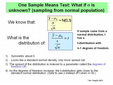
One Sample Means Test What if ? is unknown?
(sampling from normal population)
We know that
If sample came from a normal distribution, t has
a t-distribution with n-1 degrees of freedom.
What is the distribution of

• Symmetric about 0.
• Looks like a standard normal density, only more
  spread out.
• 3) The spread of the distribution is indexed to
  a parameter called the degrees of freedom (df).
• 4) As the degrees of freedom increase, the
  t-distribution gets closer to the standard normal
  distribution. (Safe to use z instead of t when
  ngt30.)

2
Tail probabilities of the t-distribution
See Table 3 Ott Longnecker
3
Rejection Regions for hypothesis tests using
t-distribution critical values
For Pr(Type I error) ?, df n - 1
H0 ? ?0
Reject H0 if t gt t?,n-1 t lt -t?,n-1 t gt
t?/2,n-1
HA 1. ? gt ?0 2. ? lt ?0 3. ? ? ?0
4
Degrees of Freedom
Why are the degrees of freedom only n - 1 and
not n?
We start with n independent pieces of information
with which we estimate the sample mean.
Now consider the sample variance
5
Confidence Interval for ? when ? unknown (samples
are assumed to come from a normal population)
with df n - 1 and confidence coefficient (1 -
?). (Can use z?/2 if ngt30.)
Example Compute 95 CI for ? given
6
The Level of Significance of a Statistical Test
(p-value)

• Suppose the result of a statistical test you
  carry out is to reject the Null.
• Someone reading your conclusions might ask How
  close were you to not rejecting?
• Solution Report a value that summarizes the
  weight of evidence in favor of Ho, on a scale of
  0 to 1. This the p-value. The larger the p-value,
  the more evidence in favor of Ho.

Formal Definition The p-value of a test is the
probability of observing a value of the test
statistic that is as extreme or more extreme
(toward Ha) than the actually observed value of
the test statistic, under the assumption that Ho
is true. (This is just the probability of a Type
I error for the observed test statistic.)
Rejection Rule Having decided upon a Type I
error probability ?, reject Ho if p-value ? ?.
7
Equivalence between confidence intervals and
hypothesis tests
Rejecting the two-sided null Ho ? ?0 is
equivalent to ?0 falling outside a (1-?)100
C.I. for ?.
Rejecting the one-sided null Ho ? ? ?0 is
equivalent to ?0 being greater than the upper
endpoint of a (1-2?)100 C.I. for ?, or ?0
falling outside a one-sided (1-?)100 C.I. for ?
with infinity as lower bound.
Rejecting the one-sided null Ho ? ? ?0 is
equivalent to ?0 being smaller than the lower
endpoint of a (1-2?)100 C.I. for ?, or ?0
falling outside a one-sided (1-?)100 C.I. for ?
with infinity as upper bound.
8
Example Practical Significance vs. Statistical
Significance
Dr. Quick and Dr. Quack are both in the business
of selling diets, and they have claims that
appear contradictory. Dr. Quack studied 500
dieters and claims, A statistical analysis of my
dieters shows a significant weight loss for my
Quack diet. The Quick diet, by contrast, shows
no significant weight loss by its dieters. Dr.
Quick followed the progress of 20 dieters and
claims, A study shows that on average my dieters
lose 3 times as much weight on the Quick diet as
on the Quack diet. So which claim is right? To
decide which diets achieve a significant weight
loss we should test Ho ? ? 0 vs. Ha ? lt 0
where ? is the mean weight change (after minus
before) achieved by dieters on each of the two
diets. (Note since we dont know ? we should do
a t-test.)
9
MTB output for Quack diet analysis (Stat ? Basic
Stats ? 1 - Sample t) One-Sample T Quack Test of
mu 0 vs mu lt 0 Variable N Mean
StDev SE Mean Quack 500 -0.913
9.744 0.436 Variable 95.0 Upper
Bound T P Quack
-0.194 -2.09 0.018 Difference Size
Power 1 500 0.6295
R output for Quick diet analysis (Read 20 values
into vector quack) gt t.test(quick,alternativec(
"less"),mu0,conf.level0.95) One Sample
t-test, data quick t -1.0915, df 19,
p-value 0.1443 alternative hypothesis true
mean is less than 0 95 percent confidence
interval -Inf 1.594617 sample estimate of
mean of x -2.73 gt power.t.test(n20,delta1,sd11
.185,type"one.sample",
alternative"one.sided") n 20, delta 1,
power 0.104
10

• Summary
• Quicks average weight loss of 2.73 is over 3
  times as much as the 0.91 weight loss reported by
  Quack.
• However, Quacks small weight loss was
  significant, whereas Quicks larger weight loss
  was not! So Quack might not have a better diet,
  but he has more evidence, 500 cases compared to
  20.
• Remarks
• Significance is about evidence, and having a
  large sample size can make up for having a small
  effect.
• If you have a large enough sample size, even a
  small difference can be significant. If your
  sample size is small, even a large difference may
  not be significant.
• Quick needs to collect more cases, and then he
  can easily dominate the Quack diet (though it
  seems like even a 2.7 pound loss may not be
  enough of a practical difference to a dieter).
• Both the Quick Quack statements are somewhat
  empty. Its not enough to report an estimate
  without a measure of its variability. Its not
  enough to report a significance without an
  estimate of the difference. A confidence interval
  solves these problems.

11
A confidence interval shows both statistical and
practical significance. Quack two one-sided 95
CIs
One-sided CI says mean is sig. less than zero.
Quick two one-sided 95 CIs
One-sided CI says mean is NOT sig. less than
zero.