
The - PowerPoint PPT Presentation
Title:
The
Description:
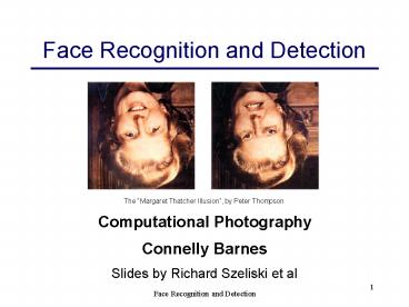
Face Recognition and Detection The Margaret Thatcher Illusion , by Peter Thompson Computational Photography Connelly Barnes Slides by Richard Szeliski et al – PowerPoint PPT presentation
Number of Views:66
Avg rating:3.0/5.0
Title: The
1
Face Recognition and Detection
The Margaret Thatcher Illusion, by Peter
Thompson
Computational Photography Connelly Barnes Slides
by Richard Szeliski et al
2
Recognition problems
- What is it?
- Object and scene recognition
- Who is it?
- Identity recognition
- Where is it?
- Object detection
- What are they doing?
- Activities
- All of these are classification problems
- Choose one class from a list of possible
candidates
3
What is recognition?
- A different taxonomy from Csurka et al. 2006
- Recognition
- Where is this particular object?
- Categorization
- What kind of object(s) is(are) present?
- Content-based image retrieval
- Find me something that looks similar
- Detection
- Locate all instances of a given class
4
Readings
- C. Bishop, Neural Networks for Pattern
Recognition, Oxford University Press, 1998,
Chapter 1. - Forsyth and Ponce, Chap 22.3 (through
22.3.2--eigenfaces) - Turk, M. and Pentland, A. Eigenfaces for
recognition. Journal of Cognitive Neuroscience,
1991 - Viola, P. A. and Jones, M. J. (2004). Robust
real-time face detection. IJCV, 57(2), 137154.
5
Sources
- Steve Seitz, CSE 455/576, previous quarters
- Fei-Fei, Fergus, Torralba, CVPR2007 course
- Efros, CMU 16-721 Learning in Vision
- Freeman, MIT 6.869 Computer Vision Learning
- Linda Shapiro, CSE 576, Spring 2007
6
Todays lecture
- Face recognition and detection
- color-based skin detection
- recognition eigenfaces Turk Pentlandand
parts Moghaddan Pentland - detection boosting Viola Jones
7
Face detection
- How to tell if a face is present?
8
Skin detection
skin
- Skin pixels have a distinctive range of colors
- Corresponds to region(s) in RGB color space
- Skin classifier
- A pixel X (R,G,B) is skin if it is in the skin
(color) region - How to find this region?
9
Skin detection
- Learn the skin region from examples
- Manually label skin/non pixels in one or more
training images - Plot the training data in RGB space
- skin pixels shown in orange, non-skin pixels
shown in gray - some skin pixels may be outside the region,
non-skin pixels inside.
10
Skin classifier
- Given X (R,G,B) how to determine if it is
skin or not? - Nearest neighbor
- find labeled pixel closest to X
- Find plane/curve that separates the two classes
- popular approach Support Vector Machines (SVM)
- Data modeling
- fit a probability density/distribution model to
each class
11
Probability
- X is a random variable
- P(X) is the probability that X achieves a certain
value
- called a PDF
- probability distribution/density function
- a 2D PDF is a surface
- 3D PDF is a volume
continuous X
discrete X
12
Probabilistic skin classification
- Model PDF / uncertainty
- Each pixel has a probability of being skin or not
skin - Skin classifier
- Given X (R,G,B) how to determine if it is
skin or not? - Choose interpretation of highest probability
- Where do we get and
?
13
Learning conditional PDFs
- We can calculate P(R skin) from a set of
training images - It is simply a histogram over the pixels in the
training images - each bin Ri contains the proportion of skin
pixels with color Ri - This doesnt work as well in higher-dimensional
spaces. Why not?
14
Learning conditional PDFs
- We can calculate P(R skin) from a set of
training images - But this isnt quite what we want
- Why not? How to determine if a pixel is skin?
- We want P(skin R) not P(R skin)
- How can we get it?
15
Bayes rule
- In terms of our problem
- What can we use for the prior P(skin)?
- Domain knowledge
- P(skin) may be larger if we know the image
contains a person - For a portrait, P(skin) may be higher for pixels
in the center - Learn the prior from the training set. How?
- P(skin) is proportion of skin pixels in training
set
16
Bayesian estimation
likelihood
posterior (unnormalized)
- Bayesian estimation
- Goal is to choose the label (skin or skin) that
maximizes the posterior ? minimizes probability
of misclassification - this is called Maximum A Posteriori (MAP)
estimation
17
Skin detection results
18
General classification
- This same procedure applies in more general
circumstances - More than two classes
- More than one dimension
- Example face detection
- Here, X is an image region
- dimension pixels
- each face can be thought of as a point in a high
dimensional space
H. Schneiderman, T. Kanade. "A Statistical Method
for 3D Object Detection Applied to Faces and
Cars". CVPR 2000
19
Todays lecture
- Face recognition and detection
- color-based skin detection
- recognition eigenfaces Turk Pentlandand
parts Moghaddan Pentland - detection boosting Viola Jones
20
Eigenfaces for recognition
- Matthew Turk and Alex Pentland
- J. Cognitive Neuroscience
- 1991
21
Linear subspaces
What does the v2 coordinate measure?
- distance to line
- use it for classificationnear 0 for orange pts
What does the v1 coordinate measure?
- position along line
- use it to specify which orange point it is
- Classification can be expensive
- Big search prob (e.g., nearest neighbors) or
store large PDFs - Suppose the data points are arranged as above
- Ideafit a line, classifier measures distance to
line
22
Dimensionality reduction
- Dimensionality reduction
- We can represent the orange points with only
their v1 coordinates (since v2 coordinates are
all essentially 0) - This makes it much cheaper to store and compare
points - A bigger deal for higher dimensional problems
23
Linear subspaces
Consider the variation along direction v among
all of the orange points
What unit vector v minimizes var?
What unit vector v maximizes var?
Solution v1 is eigenvector of A with largest
eigenvalue v2 is eigenvector of A
with smallest eigenvalue
24
Principal component analysis
- Suppose each data point is N-dimensional
- Same procedure applies
- The eigenvectors of A define a new coordinate
system - eigenvector with largest eigenvalue captures the
most variation among training vectors x - eigenvector with smallest eigenvalue has least
variation - We can compress the data using the top few
eigenvectors - corresponds to choosing a linear subspace
- represent points on a line, plane, or
hyper-plane - these eigenvectors are known as the principal
components
25
The space of faces
- An image is a point in a high dimensional space
- An N x M image is a point in RNM
- We can define vectors in this space as we did in
the 2D case
26
Dimensionality reduction
- The set of faces is a subspace of the set of
images - We can find the best subspace using PCA
- This is like fitting a hyper-plane to the set
of faces - spanned by vectors v1, v2, ..., vK
- any face
27
Eigenfaces
- PCA extracts the eigenvectors of A
- Gives a set of vectors v1, v2, v3, ...
- Each vector is a direction in face space
- what do these look like?
28
Projecting onto the eigenfaces
- The eigenfaces v1, ..., vK span the space of
faces - A face is converted to eigenface coordinates by
29
Recognition with eigenfaces
- Algorithm
- Process the image database (set of images with
labels) - Run PCAcompute eigenfaces
- Calculate the K coefficients for each image
- Given a new image (to be recognized) x, calculate
K coefficients - Detect if x is a face
- If it is a face, who is it?
- Find closest labeled face in database
- nearest-neighbor in K-dimensional space
30
Choosing the dimension K
eigenvalues
- How many eigenfaces to use?
- Look at the decay of the eigenvalues
- the eigenvalue tells you the amount of variance
in the direction of that eigenface - ignore eigenfaces with low variance
31
View-Based and Modular Eigenspaces for Face
Recognition
- Alex Pentland, Baback Moghaddam and Thad
StarnerCVPR94
32
Part-based eigenfeatures
- Learn a separateeigenspace for eachface feature
- Boosts performanceof regulareigenfaces
33
Bayesian Face Recognition
- Baback Moghaddam, Tony Jebaraand Alex Pentland
- Pattern Recognition
- 33(11), 1771-1782, November 2000
- (slides from Bill Freeman, MIT 6.869, April 2005)
34
Bayesian Face Recognition
35
Bayesian Face Recognition
36
Bayesian Face Recognition
37
Morphable Face Models
- Rowland and Perrett 95
- Lanitis, Cootes, and Taylor 95, 97
- Blanz and Vetter 99
- Matthews and Baker 04, 07
38
Morphable Face Model
- Use subspace to model elastic 2D or 3D shape
variation (vertex positions), in addition to
appearance variation
Shape S
Appearance T
39
Morphable Face Model
- 3D models from Blanz and Vetter 99
40
Face Recognition Resources
- Face Recognition Home Page
- http//www.cs.rug.nl/peterkr/FACE/face.html
- PAMI Special Issue on Face Gesture (July 97)
- FERET
- http//www.dodcounterdrug.com/facialrecognition/Fe
ret/feret.htm - Face-Recognition Vendor Test (FRVT 2000)
- http//www.dodcounterdrug.com/facialrecognition/FR
VT2000/frvt2000.htm - Biometrics Consortium
- http//www.biometrics.org
41
Todays lecture
- Face recognition and detection
- color-based skin detection
- recognition eigenfaces Turk Pentlandand
parts Moghaddan Pentland - detection boosting Viola Jones
42
Robust real-time face detection
- Paul A. Viola and Michael J. Jones
- Intl. J. Computer Vision
- 57(2), 137154, 2004
- (originally in CVPR2001)
- (slides adapted from Bill Freeman, MIT 6.869,
April 2005)
43
Scan classifier over locs. scales
44
Learn classifier from data
- Training Data
- 5000 faces (frontal)
- 108 non faces
- Faces are normalized
- Scale, translation
- Many variations
- Across individuals
- Illumination
- Pose (rotation both in plane and out)
45
Characteristics of algorithm
- Feature set (is huge about 16M features)
- Efficient feature selection using AdaBoost
- Image representation Integral Image (also known
as summed area tables) - Cascaded Classifier for rapid detection
- Fastest known face detector for gray scale images
46
Image features
- Rectangle filters
- Similar to Haar wavelets
- Differences between sums of pixels inadjacent
rectangles
47
Integral Image
- Partial sum
- Any rectangle is
- D 14-(23)
- Also known as
- summed area tables Crow84
- boxlets Simard98
48
Huge library of filters
49
Constructing the classifier
- Perceptron yields a sufficiently powerful
classifier - Use AdaBoost to efficiently choose best features
- add a new hi(x) at each round
- each hi(xk) is a decision stump
hi(x)
bEw(y xgt q)
aEw(y xlt q)
x
q
50
Constructing the classifier
- For each round of boosting
- Evaluate each rectangle filter on each example
- Sort examples by filter values
- Select best threshold for each filter (min error)
- Use sorting to quickly scan for optimal threshold
- Select best filter/threshold combination
- Weight is a simple function of error rate
- Reweight examples
- (There are many tricks to make this more
efficient.)
51
Good reference on boosting
- Friedman, J., Hastie, T. and Tibshirani, R.
Additive Logistic Regression a Statistical View
of Boosting - http//www-stat.stanford.edu/hastie/Papers/boost
.ps - We show that boosting fits an additive logistic
regression model by stagewise optimization of a
criterion very similar to the log-likelihood, and
present likelihood based alternatives. We also
propose a multi-logit boosting procedure which
appears to have advantages over other methods
proposed so far.
52
Trading speed for accuracy
- Given a nested set of classifier hypothesis
classes - Computational Risk Minimization
53
Speed of face detector (2001)
- Speed is proportional to the average number of
features computed per sub-window. - On the MITCMU test set, an average of 9 features
(/ 6061) are computed per sub-window. - On a 700 Mhz Pentium III, a 384x288 pixel image
takes about 0.067 seconds to process (15 fps). - Roughly 15 times faster than Rowley-Baluja-Kanade
and 600 times faster than Schneiderman-Kanade.
54
Sample results
55
Summary (Viola-Jones)
- Fastest known face detector for gray images
- Three contributions with broad applicability
- Cascaded classifier yields rapid classification
- AdaBoost as an extremely efficient feature
selector - Rectangle Features Integral Image can be used
for rapid image analysis
56
Face detector comparison
- Informal study by Andrew Gallagher, CMU,for CMU
16-721 Learning-Based Methods in Vision, Spring
2007 - The Viola Jones algorithm OpenCV implementation
was used. (lt2 sec per image). - For Schneiderman and Kanade, Object Detection
Using the Statistics of Parts IJCV04, the
www.pittpatt.com demo was used. (10-15 seconds
per image, including web transmission).
57
SchneidermanKanade
ViolaJones
58
Todays lecture
- Face recognition and detection
- color-based skin detection
- recognition eigenfaces Turk Pentlandand
parts Moghaddan Pentland - detection boosting Viola Jones
59
Active Shape/Appearance Models
Active Shape Models
Active Appearance Models
60
Questions?
Recommended
CrystalGraphics Presentations


