Biases associated with convenient sampling

1
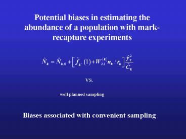
Potential biases in estimating the abundance of a
population with mark-recapture experiments
vs.
well planned sampling
Biases associated with convenient sampling
2
Ecological understanding of the population
Management
(e.g., PBR)
3
Capture-Mark-Recapture experiments and
Jolly-Seber analyses

• Basic assumptions
• Equal survival rate of all animals,
• Marks are not lost,
• Equal probability of releasing captured animals,
• Captures are instantaneous, and
• Equal capture probability of all animals.

4
Effects of sampling designs on estimates

?
5
An assumption All animals have the same
probability of being caught.

• May be violated by
• Movements of animals in and out of sampling areas
  (e.g., seasonal migration),
• Difference in individual behavior of animals, and
• Difference in capture probabilities among
  sampling areas (effort, skill, environmental
  factors, etc.).

6
Objective
To evaluate effects of various sampling designs
on abundance estimates from open population
models.
Effects of

• Assumed random movements of animals.
• Small spatial sample coverage.
• Variable capture probabilities among sampling
  areas.

7
The Simulation Model

• A simple polygon defined the population.
• The initial total abundance was 1000, of which
  200 were local residents.
• There was no birth.
• Death of an animal was a random event with the
  population annual death rate of 0.1.
• Daily movement of an animal was defined by a
  probability function.
• Behavior of each animal with respect to
  observers was defined by a probability
  function.
• Animals moved independent of each other.

8
An example of distribution of animals and
sampling areas during the simulation
Assumed coast line
9
Defining the capture probability of each
individual
Prbehavior 0.8458, 0.8132, 0.9539,
0.9610, 0.8154,
BETA(15, 2)

• Prcapture at each study area
• Fixed at 0.9.
• Fixed at 0.3.
• Locations 1 and 3 UNIF(0.1, 0.5) and Location 2
  UNIF(0.5, 0.9)
• Locations 1 and 3 UNIF(0.5, 0.9) and Location 2
  UNIF(0.1, 0.5)

Location specific capture probability
Prcapture if the first animal is in a study
area 0.8458 ? 0.9 0.7612
10
Effects of movements of animals on estimated
abundance (What if we assumed animals move
randomly?)

• A comparison of estimated abundances between two
  models
• Animals move randomly.
• Animals make seasonal migration.

• Samples were collected at Location 2 every 30
  days.
• Location specific capture probability was 0.9 or
  0.3.
• Sampling area was 10 of the entire area.

11
Random and migratory movements of animals
Random
Migratory
12
Random movements of animals
1000
800
600
Abundance (SE)
400
200
Location specific capture probability 0.9 and
0.3
0
0
50
100
150
200
250
300
350
Time (Julian days)
13
Seasonal movements of animals
1400
1200
1000
Abundance (SE)
800
600
400
Location specific capture probability 0.9 and
0.3
200
0
0
50
100
150
200
250
300
350
Time (Julian days)
14
Effects of small sample areas on estimated
abundance (What if we sampled only a fraction of
the entire area?)
The sum of sample coverage for three sampling
locations was changed from 5 to 50 of the
entire area.

• Samples were collected at three locations
  simultaneously every 30 days.
• Location specific capture probability was held
  constant at 0.9.
• Movements of animals were seasonal.

15
Location 1
Location 2
500
400
300
200
100
Mean Bias (SE)
0
-100
-200
-300
Spatial
5 (17)
10 (33)
15 (50)
20 (67)
25 (83)
30 (93)
35 (100)
40 (100)
45 (100)
50 (100)
(Coastal)
Coverage (coastal )
16
Effects of variable capture probabilities among
sampling areas on estimated abundance

• Capture probability at each sampling location was
  changed.
• Greater capture probability at Locations 1 and 3
  than at Location 2.
• Greater capture probability at Location 2 than at
  Locations 1 and 3.

• Samples were collected at three locations every
  30 days.
• 20 of the entire area was sampled.
• Movements were seasonal.

17
2500
2000
1500
Abundance (SE)
1000
1 0.612 Location specific capture
probability 2 0.251 3 0.508
500
0
0
50
100
150
200
250
300
350
Time (Julian Days)
18
1 0.149 Location specific capture
probability 2 0.835 3 0.168
1000
800
600
Abundance (SE)
400
variable capture probability model
200
death-only Jolly-Seber model
0
0
50
100
150
200
250
300
350
Time (Julian Days)
19
Conclusions for long-term sampling

• Jolly-Seber abundance estimates often
  underestimate the true abundance.

• Movements of animals should be considered before
  planning mark-recapture experiments.

• Spatial extensive sampling is more important
  than local intensive sampling.

• If observer capture probabilities are variable
  among sampling locations, the most efficient
  sampling should be conducted at locations where
  animals are present seasonally.

20
And finally This simulation model can be used
for evaluating sampling designs, when
mark-recapture experiments are considered for
abundance estimates.
21
Acknowledgments Steven Swartz (NMFS) Brenda
Smith (NMFS) Dan Goodman (Montana State
University) Bert Herting (Montana State
University) Dan Hennen (Montana State
University) Richard Jachowski (Northern Rocky
Mountain Science Center) Rick Sojda (Northern
Rocky Mountain Science Center) David Staples
(Montana State University) Mark Taper (Montana
State University) Eric Ward (Montana State
University) Chris Wright (Montana State
University)
22
Abundance
Time (Julian days)
23
1200
1000
800
Abundance
600
400
Seasonal movements of animals
Capture probability 0.9 and 0.3
200
0
0
50
100
150
200
250
300
350
Time (Julian days)