By looking back, scientists see a bright future for climate change

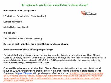
1
By looking back, scientists see a bright future
for climate change? Public release date
14-Apr-2004 Print Article E-mail Article
Close Window Contact Mary Tobin mtobin_at_ldeo.col
umbia.edu 845-365-8607 The Earth Institute at
Columbia University By looking back, scientists
see a bright future for climate change New
climate model predicted every major change For
scientists studying climate change, the past is
often a key to understanding the future. Dake
Chen at Columbia University's Lamont-Doherty
Earth Observatory recently used more than a
century of climate data to successfully test an
improved model of ENSO, the El-Niño/Southern
Oscillation that scientists believe is behind
climate change in many parts of the world. Chen
and his colleagues report in the April 15 issue
of the journal Nature that an improved climate
model, known as LDEO5, for the first time
predicted every major change in the temperature
of the tropical Pacific Ocean over the past 150
years with up to two years of advance notice. In
addition, their results suggest that ENSO is
largely driven by internal relationships between
ocean temperature and tropical winds rather than
more unpredictable factors such as externally
driven wind bursts, making the future of
long-term climate prediction much more
optimistic.
2
Predictability of El Nino Recent
Developments Francis P. A. Thanks
to Prof. B. N. Goswami CENTER FOR ATMOSPHERIC
AND OCEANIC SCIENCE Indian Institute of
Science Bangalore-12, India
3
Understanding El Nino
Strong winds during La Nina pile up the warm
water in the west, causing the thermocline to
slope downwards to the west and exposing cold
water to the surface in the east. Relaxed winds
during El Nino permit the warm water to flow back
eastward so that the thermocline becomes more
horizontal. The trade wind fluctuations are both
the cause and consequence of the sea surface
temperature variations. The ocean-atmosphere
interactions permit a variety of natural modes of
oscillation. The phenomena observed in the
tropical Pacific presumably correspond to one of
or some combination of those modes.
4
TOGA Array
5
Normalized time series of SST anomaly over Nino 3
area (blue) and Southern Oscillation Index (SOI,
red). Nino 3 region 150W-90W-5S-5N
6
Understanding El Nino
Despite these considerable observational and
theoretical advances over the past few decades,
many issues are still being debated, and each El
Nino still brings surprises. The prolonged
persistence of warm conditions in the early 1990s
was as unexpected as the exceptional intensity of
El Nino in 1982 and again in 1997 nobody knew
what to expect of El Nino in 2002.
Following are the major issues related
to ENSO Why is the observed ENSO so irregular?
How predictable is El Nino? What are
the reasons for the decadal modulation of El
Nino, the apparent change in its properties
that occurred in the 1970s? How will global
warming influence El Nino? Various investigators
have different views on these issues. In this
review, we focus on the predictability of ENSO
Why are different El Nino episodes so different,
and so difficult to predict?
7
Understanding El Nino
The current disagreements concerning El Nino
have their origins in the recent history of
research on the phenomenon. When the available
datasets were scant, during the 1960s and 1970s,
we regarded El Nino as a departure from normal
conditions, as the response of the coupled
ocean-atmosphere to certain triggers. This
implied that measurements should be made during
the abnormal or anomalous periods when El Nino
happens to appear in the Pacific, the way
meteorologists make special efforts to observe
hurricanes when those cyclones appear. Wyrtki
(1975) tentatively identified a sudden collapse
of the trade winds as the most important trigger,
but intense El Nino of 1982 was not preceded by
such a collapse. The availability of more
detailed wind datasets in the 1980s led to the
identification of sporadic westerly wind bursts
that last for a few weeks along the equator in
the neighborhood of the dateline as important
triggers of El Nino. Such bursts contributed to
the development of El Nino in 1997, but similar
bursts on other occasions failed to have a
similar effect. There must be more to the story
than westerly wind bursts. The availability,
in the 1980s, of relatively long time-series
similar to those in Figure 2 prompted some
investigators to question whether each El Nino is
an independent, transient phenomenon in response
to a trigger, with a definite beginning followed
by growth and, finally, decay. Instead, they
adopted a radically different perspective and
regarded El Nino as part of a continual
oscillation without a beginning or end. El Nino
therefore has a complement, usually referred to
as La Nina. Conditions in the Pacific correspond
either to the one or the other very seldom are
conditions normal, as is evident in Figure 2.
The main challenge is not to identify triggers
but to explain the properties of the oscillation,
its period, spatial structure, etc. This new
perspective implied a different measurement
strategy. Sporadic measurements when the
phenomenon happens to appear gave way to arrays
of instruments, for example, the one in Figure 1
that monitors the tropical Pacific
continuously. Philander and Fedorov, Is El
Nino Sporadic or cyclic? Ann. Rev. Earth Planet.
Sci. (2003)
8
Understanding El Nino
It appears that ENSO has a periodicity of 3-7
years Intensity of different events are very
different There is longer time scale (of
decades or more) variations also
9
Now let us look at the irregularities in
ENSO episodes with the help of an idealized
coupled ocean-atmosphere model (Neelin 1990)
without weather or random atmospheric
disturbances-essentially to analyze the effect of
ocean atmospheric coupling. a) Weak coupling
ENSO is a damped oscillation. Initial westerly
wind burst lasting one month generated ENSO
conditions but decayed fast. b) Moderate
coupling ENSO becomes a self sustaining
oscillation. c) Intense coupling ENSO grows
to such a large amplitude that secondary
instabilities also appear. Which panel
corresponds to reality?
10
Which panel corresponds to reality? Some
investigators favor the right-hand panel. In
that case, the Southern Oscillation is similar to
weather in having as its source of irregularity
not externally imposed disturbances, but internal
nonlinear processes. However, there is
persuasive evidence that random atmospheric
disturbances, for example, westerly wind bursts
along the equator in the neighborhood of the
dateline, influence the development of El Nino on
some occasions, as happened in 1997 (McPhaden
Yu 1999). Because of such observations, some
scientists believe that the Southern Oscillation
is damped and is sustained by noise so that the
left-hand panel is the realistic one. If that
were the case, then each El Nino would be
independent of the next and would depend, for its
initiation, on noise. It is then difficult to
explain why very similar westerly wind bursts
lead to the development of El Nino on some
occasions but not others, and why the Southern
Oscillation has a distinctive timescale of a few
years. A compromise that accommodates the
various points of view posits that the Southern
Oscillation is weakly damped and is sustained by
random disturbances the panel in Figure that
corresponds to reality is then midway between the
one on the left and the central one.
11
Predictability of El Nino The Southern
Oscillation involves phenomena with two
timescales an oscillation with a period of
several years and rapid developments over a
period of weeks or months in response to random
disturbances. Hence, it should be possible to
anticipate certain aspects of the Southern
Oscillation far in advance. For example,
since the 1980s, the intensity of El Nino has
varied enormously from one event to the next, but
the phenomenon has nonetheless appeared with
remarkable regularity every five years, in 1982,
1987, 1992, 1997, and 2002.
A useful analogy for the Southern Oscillation is
a slightly damped, swinging pendulum sustained by
modest blows at random times. In the absence of
noise, El Nino would be perfectly predictable
because the Southern Oscillation would be
perfectly periodic while its amplitude slowly
attenuates. Noise sustains the oscillation and
makes it irregular. The initial conditions do
matter because they describe the phase of the
Southern Oscillation and strongly influence the
impact of random disturbances. For example, a
burst of westerly winds when the oscillation
enters its El Nino phase is very different from
the impact of the same winds when the oscillation
enters its La Nina phase.
L
Fedorov, Harper, Philander, Winter, and
Wittenberg, BAMS (2003)
12
Predictability of El Nino
The above discussion thus emphasize the
importance of atmospheric noise, particularly the
so-called westerly wind bursts in the western
equatorial Pacific. In such a scenario, ENSO is a
damped oscillation sustained by stochastic
forcing, and its predictability is more limited
by noise than by initial errors. This implies
that most El Nino events are essentially
unpredictable at long lead times, because their
development is often accompanied by
high-frequency forcing. On the other hand,
several other studies such as Cane et al (1986),
Cane and Zebiak (1988), Barnet (1984), Barnet et
al (1988), Graham et al (1987) attempted to model
past El Nino events and the results were
encouraging that the El Nino events could have
been predicted well in advance indicating that
the so called 'westerly wind bursts' has only
secondary importance.
13
Predictability of El Nino
Inspired from these efforts, Goswami and Shukla
(1991) tried to determine the limits on the
predictability of the coupled ocean-atmosphere
system using the coupled model of Zebiak and Cane
(1987) for a period of 1970-1988. In this model
the initial conditions for ocean are model
simulations forced by observed wind
stress. Major results 1. The predictions
starting in the boreal winter have better skill
than those starting in spring or summer. 2.
Limiting factor of predictability is the growth
of small errors in the coupled model which is
governed by processes with two different time
scales- the faster time scale process has an
error doubling time of about 5 months while the
slower time scale has a doubling time of about 15
months. 3. It is suggested that the existence of
slow growing process gives some hope for
predictability and its success will depend on the
ability to identify initial conditions that are
insensitive to the faster growing process. 4. It
is proposed that the fast error growth result
from the coupled instability in the ZC model,
while the slow error growth is associated with
the low frequency mode of the system.
14
Predictability of El Nino
Hence we have two different views about the
limiting factors of potential predictability of
El Nino 1) The high frequency westerly wind
bursts Which are highly unpredictable 2)
Growth of initial errors Which can be overcome
by identifying initial conditions that are
insensitive to faster growing processes In
the light of this background knowledge we look in
to the 'retrospective model forecasts' by Chen et
al., 2004.
15
Retrospective predictions of El Nino and La Nina
in the past 148 years (6month lead)- Chen et al
2004.
Kaplan SST
Model
Most of the major El Nino events are
predicted Spatial structure of the events are
also well predicted.
16
Correlation of predicted anomalies with observed
anomalies (as function of lead time) for
consecutive 20yr periods 1. Skill is
relatively high for the period 1876-1895
and 1976-1995. 2. Skill is relatively poor for
the period 1916-1955. 3. The high rms error
and low correlations during 1916-1955 is
attributed to relatively less number of ENSO
events during this period.
17
Long-lead forecasts for six of the largest warm
episodes
In all cases, the model was able to predict the
observed strong El Ninos two years in advance,
though some errors exist in the forecasted onset
and magnitude of these events. The implication
is that the evolution of major ENSO events is
largely determined by oceanic initial conditions,
and that the effect of subsequent atmospheric
noise is generally secondary. It is interesting
to note that the model predicts the strong El
Nino events in the late nineteenth century, which
are notorious for their global impact. These
events have been implicated 22 in the deaths of
tens of millions of people in India, China,
Ethiopia, Northeast Brazil and elsewhere. (The
disastrous failure of the Indian monsoon in 1877
prompted the establishment of the Observatory in
India, later the venue for the work of Walker
that forms the foundation of modern understanding
of ENSO.) The predictions shown here are, to
our knowledge, the first successful retrospective
forecasts of these significant historic events.
Observed Nino 3.4
15 Months
21 Months
18 Months
24 Months
18
Summary 1. It is believed that the limiting
factors of potential predictability of El Nino
are the high frequency westerly wind bursts
Which are highly unpredictable and growth of
initial errors which can be overcome by
identifying initial conditions that are
insensitive to faster growing processes. 2. Chen
et al show that the predictions depend more on
initial conditions that determine the phase of
ENSO, than on unpredictable atmospheric noise.
3. Although westerly wind bursts do affect the
exact onset time and perhaps the amplitude of El
Nino, the gross features of ENSO seem to be coded
in the large-scale dynamic state. 4. These
results favour the interpretation that the
enhanced wind burst activity in the boreal spring
preceding large El Nino events is consequence of
those ongoing events rather than a cause. 6.
A practical consequence of our results is a more
optimistic view of the possibility of
skillful long-lead forecasts of El Nino.
19
Methods The model used in this study, called
LDEO5, is the latest version of an intermediate
ocean atmosphere coupled model widely applied to
ENSO investigation and prediction. It differs
from its predecessor LDEO4 in its improved
ability to assimilate SST data, which is crucial
here as only reconstructed SST data sets are
available for such a long-term experiment. In
LDEO5, an assimilated SST field not only directly
affects the surface wind field as in LDEO4, but
also has a persistent effect on the coupled
system. The improvement was achieved by including
a bias correction term in the model SST equation
that statistically corrects for model
deficiencies in parameterizing subsurface
temperature and surface heat fluxes. The
correction was estimated inversely by fitting
model SST tendency to observation using data from
1980-2000, and a regression relating this term to
the multivariate model state was obtained in the
space of empirical orthogonal functions. Based on
this regression, an interactive correction of SST
was then implemented in the model. The internal
variability of LDEO5 is similar to that of LDEO4
it generates a self-sustaining oscillation with
periods of 3-5 yr and amplitudes close to those
of observed El Nino's. However, the new version
has a higher predictive skill when multiple data
sets- sea level, winds, SST are used for
initialization, and its skill decreases only
slightly when assimilating only SST data. We
have to rely on SST data here because tropical
Pacific sea level observations are virtually
non-existent before 1970, and historic wind
information is sparse and poorly calibrated.
20
Note that in the coupled initialization procedure
of the LDEO forecast system, assimilated SST data
are not simply putting a constraint on the ocean
model with SST observations they translate to
surface wind field and subsurface ocean memory.
The SST data set used in this study is the
reconstructed analysis for the extended period of
1856-2003. Initialized with this monthly
analysis, a forecast with lead times up to 24
months was made from each month of the 148-yr
period. The same data set was also used to
verify the model predictions.