4' Standard Regression Model and Spatial Dependence Tests

1
4. Standard Regression Model and Spatial
Dependence Tests
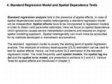
Standard regression analysis fails in the
presence of spatial effects. In case of spatial
dependencies and/or spatial heterogeneity a
standard regression model will be misspecified.
Spatial effects have to be incorporated in
regression models in order to obtain valid
parameter estimates. Here we focus on spatial
dependence which ignorance causes severe
interpretation problems and requires an
original spatial modelling approach. Spatial
heterogeneity can much more be accounted for by
methods developed in mainstream
econometrics. The standard regression model is
usually the starting point of spatial
regression analysis. The residuals of ordinary
least-squares (OLS) estimation can be used
to test for spatial effects. Hence, we first
outline OLS estimation in the standard regression
model. The most frequently used spatial models,
the spatial lag mo del and the spatial error
model, are presented in sections 4.2 and 4.3.
Various Tests for spatial effects are introduced
in chapter 5.
2
4.1 The standard regression model
Linear regression model Relationsship between a
dependent variable Y and a set of explanatory
variables X1, X2, , Xk.
(4.1)
nx1 vector of the dependent variable
nxk matrix with observations of the k
explanatory variables
xij observation of the jth variable at the ith
statistical unit 1st column of X vector of ones
(for intercept) The explanatory variables are
treated as fixed and not random.
kx1 vector of regression coefficients
nx1 vector of disturbances (error terms)
3

• ? Standard assumptions
• The disturbance has an expection of zero
• for all i
• The disturbances have a constant variance
  (homoscedasticity)
• for
  all i, ?2 error variance
• The disturbances are uncorrelated (lack of
  autocorrelation)
• 
  for all i?j

Assumptions 1-3 in compact form
and
o nx1 vector of zeros, I nxn identity matrix
For carrying out statistical tests normality of
the errors is assumed
for all i or
4
? Ordinary least squares (OLS) estimation An
important task of regression analysis is to
estimate the unknown vector of re- gression
coefficients, ß, in order to assess the influence
of the regressors X1, X2, , Xk on the dependent
variable Y. Under the standard assumptions,
ordinary least squares (OLS) estimation yields
best linear unbiased estimators (blue
pro- perty). Least squares criterion (4.2a)
Q has to be minimized with respect to ß for
which we use the equivalent expression (4.2b)
First order condition for a minimum of
Q OLS estimator of ß (4.3)
5
? Fitted values, residuals and residual
variance Fitted values (4.4) Residuals (4.5a)
or (4.5b) Residual variance
(unbiased estimate of ?2) (4.6)
( )

Standard error of regression (SER) (4.7)
6
? Measures of fit Decomposition of the total sum
of squares of the dependent variable Y (4.8)
SST SSE SSR Total sum of squares (4.9) Exp
lained sum of squares (4.10) Residual sum of
squares (4.11) Coefficient of determination
(4.12a) or (4.12b)
Range of R2 0 R2 1
7

• Adjusted coefficient of determination
• By the adjustment regression models with
  different numbers of regressors are made
  comparable.
• (4.13)
• Information criteria
• Information measure the goodness of fit whereat
  model complexity in terms of
• the number of explanatory variables is penalized.
  Goodness of fit is covered by the log likelihood
  function ln(L) which is mainly composed of the
  sum of squared residuals. By penalizing fits with
  a larger number of regressors, re-gression
  models with different k are made comparable.
  According to the infor-mation criteria, the model
  with the lowest value is the best.
• - Akaike information criterion (AIC)
• (4.14) AIC -2?ln(L) 2k
• Schwartz criterion (SC)
• (4.15) SC -2?ln(L) k?ln(n)

8

• ? Hypothesis tests
• Test of significance of regression coefficients
• Null hypothesis H0 ßj 0
• Distribution of the OLS estimator under H0
  for normally distributed errors
• Test statistic
• (4.16)
• xxjj jth main diagonal element of the inverse
  (XX)-1
• tj follows a t distribution with n-k degrees
  of freedom.
• Significance level a
• Critical value (two-sided test) t(n-k1-a/2)

9

• F test for the regression as a whole
• Null hypothesis H0 ß2 ß3 ßk 0
• SSRc Constrained residual sum of squares from
  a regression in which H0 holds
• i.e. a regression of Y on the
  constant term X1 only
• SSRu Unconstrained residual sum of squares
  from a regression of Y on X1, X2,
• , Xk
• Test statistic
• (4.17a)
• or
• (4.17b)

10
Example For 5 regions are data available on
output growth (X) and productivity growth (Y)
According to the Verdoorn law output growth and
productivity growth are posi- tively related.
Productivity growth increases with output growth
due to increasing returns to scale. The
regression model implied by Verdoorns law
reads (4.18) with xi11 for all i and xi2 xi.
If Verdoorns law holds, the Verdoorn
coefficient ß2 is expected to take a positive
sign. The intercept captures productivity growth
evoked by autonomous technical progress. The
regression model (4.17) can be estimated by OLS.
11
Vector of the endogenous variable y
Observation matrix X
Matrix product XX, its inverse (XX) -1, matrix
product Xy
,
,
OLS estimator of ß
12
Vector of fitted values
Vector of residuals e
13
Residual variance
Standard error of regression (SER)
14
Coefficient of determination
Working table ( )
SST 0.4520, SSE 0.4132, SSR SST SSE
0.4520 -0.4132 0.0388
or
15
Test of significance of regression coefficients
- for ß1 (H0 ß1 0)
OLS estimator for ß1
Test statistic
Critical value (a0.05, two-sided test)
t(3,0.975) 3.182
Testing decision ( t1 1.779) lt
t(30.975)3.182 gt Accept H0
- for ß2 (H0 ß2 0)
OLS estimator for ß2
Test statistic
Critical value (a0.05, two-sided test)
t(3,0.975) 3.182
Testing decision ( t2 5.643) gt
t(30.975)3.182 gt Reject H0
16
F test for the regression as a whole Null
hypothesis H0 ß2 0 (only one non constant
exogenous variable)
Constrained residual sum of squares SSRc SST
0.4520 Unconstrained residual sum of squares
SSRu SSR 0.0388
Test statistic
or
(The difference of both computations of F are
only due to rounding errors.)
Critical value(a0.05) F(130.95) 10.1
Testing decision (F31.948) gt F(130.95)10.1
gt Reject H0