5. Spatial regression models 5.1 Basic types of spatial regression models

1
5. Spatial regression models5.1 Basic types of
spatial regression models

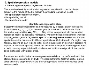
• There are two basic types of spatial regression
  models which can be chosen
• subject to the results of the LM tests in the
  standard regression model
• - the spatial cross-regressive model,
• the spatial lag model,
• the spatial error model.

Spatial
cross-regressive Model Substantive spatial
dependence can be captured by a spatial lags in
the explora- tory variables X2, X3, , Xk or the
endogenous variable Y. In the former case, the
spatial lag variables Wx2, Wx3, , Wxk will be
incorporated into the standard regression model
as additional regressors. We term the regression
model with spa- tially lagged exogenous
regressors spatial cross-regressive model.
Substantive spatial interaction can occur in
different applications. Output growth of a region
may Not only depend on own regions initial
income but as well on income in adjacent
re- regions. In this case, spillover effects are
restricted to neighbourhood regions. Such a
restriction may especially hold for spillovers of
tacit knowledge which is expected to be exchanged
within local areas. Parameter estimation in the
cross-regressive model can be performed as in the
standard regression model by OLS. This results
from the fact that spatial lag vari- ables share
the properties with the original regressors,
which are assumed to be non-stochastic.
2

Spatial lag model The spatial lag model captures
as well substantial spatial dependencies like
external effects or spatial interactions. It
assumes that such dependencies mani-fests in the
spatial lag Wy of the dependent variable Y.
Regional growth may be fostered by growth in
neighbourhood regions by flows of goods for
example. In this case, spillover effects are not
restricted to adjacent regions but propagated
over the entire regional system. In
accordance to the the time-series analogue the
pure spatial lag model is also termed spatial
autoregressive (SAR) model. In applications the
model also in- corporates a set of explanatory
variables X1, X2, , Xk. This extension is
ex-pressed by the term mixed regressive, spatial
autoregressive model. In all instances OLS
estimation will produce biased and inconsistent
parameter esti-mates, we introduce the method of
instruments (IV method) and the method of maximum
likelihood (ML method) as adequate estimation
methods for that type of model. Because only the
spatial lag Wy is relevant for the choice of an
alternative estimation method to OLS, the term
spatial lag mo-del is often kept in cases where
the model is extended by exogeneous X-variables.

3

Spatial error model The spatial error model is
applicable when spatial autocorrelation occurs
as nuisance resulting form misspecification or
inadequate delineation of spatial units.
Unmodelled interaction among regions are
restricted to the error terms. In convergence
studies, the convergence rate will be properly
assessed by sta- dard estimation methods.
However, a random shock occurring in a specific
region Is not restricted to that region and its
neighbourhood but will diffuse across the entire
regional system. Spatial dependence in for of
nuisance entails that the disturbances ei are no
longer independently identically distributed
(i.i.d.), but follow an autoregressive (AR)
or moving average (MA) process. In analogy to the
Markov process in time-series analysis, the
disturbance term is assumed to folllow a first
order autoregressive (AR) process in the spatial
error model. In consideration of the explanation
of the dependent variable Y by a set of
exogenous variables X1, X2, , Xk, the spatial
error model serves as an abbreviation for a
linear regression model with a spa- tial
autoregressive disturbance. In contrast to
substantial dependence, spatial dependence in
form of nuisance does not entail inconsistency
of OLS estimated regression coefficients.
However, As their standard errors are biased,
significance tests based on OLS estimation can
be misleading. In order to allow for valid
inference, other estimation principles
4
must adopted. We outline maximum likelihood (ML)
estimation in the spatial error model. An
alternative is provided by Kelejian and Prucha
(1999) in form of a General Moment (GM) estimator
which is not dealt with in our introductory
course.
Specification tests The presence of spatial
error autocorrelation can be assessed by the
Moran test applied on the residuals of the
standard regression model (see section 4.2). This
omnibus test does, however, not point to a basic
spatial model. No specific spatial test is
available for the spatial cross-regressive model.
Florax and Fol-mer (1992) suggest to apply the
well-known F-test for linear restrictions on the
regression coefficients to identify spatial
autocorrelation due to omitted lagged exogenous
variables. This test requires the estimation of
both the restricted and the unrestricted
regression model. For the two other type of
spatial models Lagrange Multiplier (LM) tests
that are tailured for the special spatial
settings are available - the LM lag test and
- the LM error test.
5
Both tests have to be performed after estimating
the the standard regression mo-del (see section
4.2). If the test statistic LM(lag) turns out to
be significant, but LM(error) is insignificant,
spatial autocorrelation appears to be
substantial, which means that the spatial lag
model is viewed to be appropriate. In the
converse case the spatial error model will be a
sensible choice for analysing the relation-ship
between Y and the X-variables. When both test
statistics, LM(lag) and LM(error) prove to be
significant, the test statistic with the higher
significance, i.e. the lower p-value, will guide
the choice of the spatial regres-sion model.
Ac-cording to this rule, in case of pLM(lag)
lt pLM(err) the spatial lag model will be
chosen, whereas for pLM(err) lt
pLM(lag) the spatial error model will be the
preferable spatial setting.
6
5.2 The spatial cross-regressive model
The spatial cross-regressive model presumes that
the exploratory variables X2, X3, , Xk as well
as their spatial lags LX2, , LXk influence a
geo-referenced dependent variable Y. In this
approach Y is not only affected by values
variables take in the same region but also the
take in neighbouring regions
(5.1)
y is an nx1 vector of the endogenous variable Y,
xj an nx1 vector of the exoge- nous variable Xj
(where x1 is a vector of ones for the intercept),
W an nxn spatial weight matrix and e an nxn
vector of disturbances. The parameters ßj j1,
2,,k denote theregression coefficients of the
exogenous variables X1, X2, , Xk and the
parameters ?j the regression coefficients of the
exogneous spatial lags Wx2, , Wxk. The
disturbances ei are assumed to meet the standard
assumptions for a linear regression model (see
section 4.1) expection of zero, constant
variance s² and absence of autocorrelation. For
statistical inferences like significance tests we
additionally assume the disturbances to be
normally distributed.
7
A more compact form of the spatial
cross-regressive model reads
(5.2)
.
nxk matrix with observations of the k
explanatory variables
(n-1)xk matrix with observations of the k-1
lagged explanatory variables
kx1 vector of regression coefficients of exognous
variables
(k-)x1 vector of regression coefficients of
lagged exognous variables
OLS estimator of the regression coefficients
Variance-covariance matrix of OLS estimator

8

• F test on omitted spatially lagged exogenous
  variables
• Test of the spatially lagged variables for a
  relevant subset S of X-variables one
• at a time
• Null hypothesis H0 ?j 0 for subset Xj e S
• SSRc Constrained residual sum of squares from
  a regression in which H0 holds
• i.e. a regression of Y on the
  original exogenous variables X1, X2, , Xk
• SSRu Unconstrained residual sum of squares
  from a regression of Y on the
• original exogenous variables X1, X2,
  , Xk and the spatially lagged exo-
• genous variable LXj
• Test statistic
• (5.3)

9
Generalisation of the F test Instead of testing
the spatially lagged variables of the subset S
one at a time, they can also be tested
simultanously Null hypothesis H0 All regression
coefficients ?j of the X-variables of the
subset S are equal to
zero Test statistic (5.4) q number of
X-variables in the subset S (when all X-variables
without the vec- tor of one are included in
S, q is equal to k 1) F follows an F
distribution with q and n-k degrees of freedom.
Testing decision F gt F(qn-k-q1-a) gt
Reject H0
or p lt a gt
Reject H0
10
Example In order to illustrate the spatial
cross-regressive model, we refer to the
example of 5 regions for which data are available
on output growth (X) and productivity growth (Y)
The cross-regressive model presumes that
productivity growth in region i does Not only
depend on own regions output growth but as well
on output growth in adjacent regions (5.5) with
xi11 for all i and xi2 xi. When LX captures
technological externalities from neighbouring
regions ?2 is expected to take a positive sign.
When output growth X can be treated as as
exogenous variable, the spatial lag variable LX
is as well exogneous, because the spatial weights
are determined a priori. Thus, the spatial
regression model (5.5) can be estimated by OLS.
11
Vector of the endogenous variable y
Standardized weights matrix W
Matrix of original x-variables X
Matrix of spatially lagged endogenous variables
X
Observation matrix X X
12
Matrix product X XX X
Matrix product X Xy
Inverse (X XX X)-1
OLS estimator of the regression coefficients
13
Vector of fitted values
Vector of residuals e
14
Residual variance
Standard error of regression (SER)
Estimated variance-covariance matrix of

15
Coefficient of determination
Working table ( )
SST 0.4520, SSE 0.4344, SSR SST SSE
0.4520 -0.4344 0.0176
or
16
Test of significance of regression coefficients
- for ß1 (H0 ß1 0)
OLS estimator for ß1
Test statistic
Critical value (a0.05, two-sided test)
t(2,0.975) 4.303
Testing decision ( t1 0.144) lt
t(20.975)4.303 gt Accept H0
- for ß2 (H0 ß2 0)
OLS estimator for ß2
Test statistic
Critical value (a0.05, two-sided test)
t(2,0.975) 4.303
Testing decision ( t2 5.018) gt
t(20.975)4.303 gt Reject H0
17
Test of significance of regression coefficients
- for ?2 (H0 ?2 0)
OLS estimator for ?2
Test statistic
Critical value (a0.05, two-sided test)
t(2,0.975) 4.303
Testing decision ( t1 1.560) lt
t(20.975)4.303 gt Accept H0
18
F test for the regression as a whole Null
hypothesis H0 ß2 ?2 0
Constrained residual sum of squares SSRc SST
0.4520 Unconstrained residual sum of squares
SSRu SSR 0.0176
Test statistic
or
(The difference of both computations of F are
only due to rounding errors.)
Critical value(a0.05) F(220.95) 19.0
Testing decision (F24.682) gt F(220.95)19.0
gt Reject H0
19
F test on omitted spatially lagged exogenous
variables Null hypothesis H0 ?2 0
Constrained residual sum of squares (regression
of Y on X1 (constant) and X2) SSRc SST
0.0388 (see sect. 4.1 ? standard regression
model) Unconstrained residual sum of squares
(regression of Y on X1 (constant), X2 and LX2)
SSRu SSR 0.0176
Test statistic
Critical value(a0.05) F(120.95) 18.5
Testing decision (F2.409) lt F(120.95)18.5
gt Accept H0