The Taguchi Loss Function and the Definition of Optimal

1

• The Taguchi Loss Function and the Definition of
  Optimal Performance

2
The Taguchi Loss Function and the Definition of
Optimal Performance

• A primary goal of management in any organization
  should be the effective allocation of resources
  aimed at optimizing the performance of the
  processes entrusted to them.
• Given this goal the obvious question to ask is,
  how can optimal performance be defined and
  achieved in a practical sense?
• The answer to this question is based on the
  application of Shewharts theory of variation
  already presented combined with the concept known
  as the average loss function developed by Dr.
  Genichi Taguchi.

3
The Concept of "Ideal Performance

• Consider any process for which a performance
  characteristic X is routinely measured which
  characterizes the performance of the process.
• Let T denote the target value for X, such that
  the ideal performance is defined as X T.
• That is, the process is operating in an ideal
  state if it always produces its output with the
  performance characteristic identically equal to
  the target value T with no variability.

4
The Employee Attendance Example

• Consider employee attendance within any process.
  Let X equal the percent of scheduled work hours
  that an employee actually works during the pay
  period. The target value for X is T 100, and
  ideal performance would be defined as perfect
  attendance. That is, X 100 for every
  employee for every pay period.

5
The Patient Transport Example

• Consider a patient transport process, and let V
  equal the variance from target arrival time in
  the ancillary unit. The target value for V is
  clearly T 0, and ideal performance would be
  defined as every transport completed with
  variance from target arrival time V 0 minutes.

6
The Medication Ordering Example

• Consider the process of filling medication orders
  in a pharmacy. Let X equal the daily error rate
  associated with filling the orders. In this case
  the target value for X is T 0, and the ideal
  performance is X 0. That is, the process
  produces no medication errors.

7
The Accounts Payable Example

• Consider an accounts payable process, and let X
  equal the number of days it takes to pay a vendor
  once the invoice is received. Suppose the terms
  of payment are 30 days upon receipt. The target
  number of days to pay might be T 30 days, and
  ideal performance would be defined as paying
  every invoice at exactly 30 days from receipt of
  invoice.

8
The Cup Weight Example

• Consider the HD-2 filling process. Let X equal
  the net weight of a cup filled by the process.
  In this case the target value might be T 240
  grams, and ideal performance is X 240 grams.
  That is, the machine fills every cup with exactly
  240 grams of product.

9
The Concept of "Ideal Performance

• It should be obvious that in practice ideal
  performance can never be achieved.
• This is because in the ideal state there is no
  variation in process performance, and therefore
  the performance of the process is totally
  predictable.
• But the axiom of variation does not allow for
  such an ideal state to exist, and therefore a
  search must be made for a more practical view of
  optimal process performance.

10
The Taguchi Loss Function - L(x)

• Consider any process for which the performance
  characteristic X is measured on the process
  output, and let T denote the target value for X.
  
• Further assume that the process is in a state of
  statistical control about an average or mean
  value denoted by µ, and with a standard deviation
  denoted by ?.
• Although it may not be known exactly, it is
  reasonable to assume that some economic loss is
  incurred for each individual output X, and that
  the loss depends upon the deviation of the
  measured output from target (i.e., on the
  difference X-T).

11
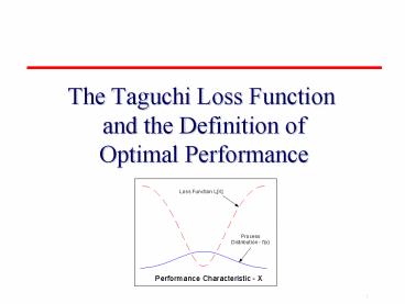
The Taguchi Loss Function - L(x)

• In mathematical terms, the loss associated with X
  can be expressed as a function of X, denoted by
  L(X), with the following general properties.
• 1) L(T) 0 i.e., the loss is minimized
  when X T
• 2) L(X) increases as X deviates
• from T.

Figure 7.1. A Typical Loss Function
12
The Average or Expected Loss - EL(x)

• Because of the variation in process performance,
  the value of the performance characteristic X is
  not constant.
• If the process is operating in a state of
  statistical control, however, the behavior of X
  is characterized by a single statistical
  distribution (i.e., the process distribution).

13
The Average or Expected Loss - EL(x)

• Figure 7.2 illustrates the relationship between
  the loss function L(X) and the process
  distribution.

Figure 7.2. Relationship Between L(X) and f(X)
14
The Average or Expected Loss - EL(x)

• Although it is beyond the scope of this book, it
  can be shown that the expected loss as defined
  above reduces to
• ELoss k?2 (? - T)2 .
• The important summary points resulting from this
  fairly complex mathematical analysis are the
  following.
• For any process that is in a state of statistical
  control, the average loss incurred over time is
  directly proportional to the process variance
  plus the square of the deviation of the process
  mean from the target value.

15
The Average or Expected Loss - EL(x)

• These results have great practical, as well as
  theoretical, value. Note that the value for the
  unknown proportionality constant K is not
  important. No matter what K equals, the average
  loss is minimized by minimizing ?2 and (µ-T)2.
  Therefore, we can assume for convenience that K
  1.
• The loss function concept clearly demonstrates
  that for any process and any loss function L, in
  order to control and minimize the average loss
  over time, focus must be placed on
• 1) bringing the process into statistical
  control
• 2) bringing the process mean on target (i.e.,
  moving µ as close as possible to T) and
• 3) minimizing the process variance ?2.

16
The Average or Expected Loss - EL(x)

• It is this analysis that has led to the new
  definition of world class quality as on-target
  with minimum variance, and to the operational
  definition of optimal performance.

17
The Definition of Optimal Performance

• The average loss function concept leads directly
  to the following practical, operational
  definition of "optimal performance."
• A Process . . . is operating in an optimal
  manner if
• 1) the process is operating in a state of
  statistical control
• 2) the process mean has been brought as close to
  the target value T as is physically and
  practically possible and
• 3) the process standard deviation has been
  reduced to the economically minimum value.

18
Estimating the Average Loss

• The average loss function is estimated using the
  measured values of the performance characteristic
  X obtained routinely from the process, and the
  summary statistics used to create the process
  control charts.
• The data are first used to establish that the
  process is in a reasonable state of statistical
  control by creating average and range charts, or
  average and standard deviation charts.
• If the control charts indicate that the process
  is in control, then let
• denote the center line for the average chart and
  or denote the center line for the range
  or S chart.

19
Estimating the Average Loss

• Letting K 1, the average loss function is then
  estimated by either

20
The Patient Transport Example

• Consider the patient transport example, and let
  the target value be T 15 minutes. A study was
  conducted in which the total transport time was
  tracked on 120 consecutive transports.
• Figure 7.3 is the histogram of the transport
  times. The trips were ordered chronologically
  and placed into rational subgroups of size n5.
  The average and range charts were constructed,
  and they are presented in Figure 7.4 which
  indicates that the process is in statistical
  control

21
The Patient Transport Example
Figure 7.3. Histogram of Patient Transport Times
Figure 7.4. Control Charts for Transport Times
22
The Patient Transport Example

• Based on these charts, the process mean µ, and
  the process standard deviation ? are estimated
  by
  minutes,
  respectively. Therefore, the average loss is
  estimated to be

23
The Patient Transport Example

• In this case the inherent process variation
  (i.e., ? 2) accounts for (62.29/82.72) x 100
  75 of the economic loss in the transport
  process. The amount by which the process mean is
  off target contributes only 25 to the loss.
• Therefore, management should first address those
  factors causing variation in the transport time
  from trip to trip, and redesign the process with
  the primary goal of reducing the variation in the
  process. A secondary concern should be moving
  the average transport time closer to the 15
  minute target.

24
Loss Function Analysis ofCup Compression
Strength Exercise

• The compression strength of plastic cups created
  by a thermoforming process is a critical
  performance characteristic. If the compression
  strength is too low then the cups will crush when
  stacked in pallets.
• Engineering studies determined that the
  compression strength of an individual cup must
  exceed 60 lbs to enure that the cup will not
  crush when stacked in pallets.
• Perform a loss function analysis on compression
  strength using the data presented in Table 7.1.

25
Loss Function Analysis ofCup Compression
Strength Exercise
Table 7.1. Cup Compression Strength Data