
Moving past vision, to understand motion and video. - PowerPoint PPT Presentation
1 / 21
Title:
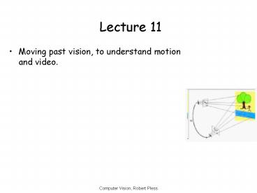
Moving past vision, to understand motion and video.
Description:
In the presence of noise, all methods to compute optic flow from images gives a bias. ... distribution leads to different biases in the computed optic flow. ... – PowerPoint PPT presentation
Number of Views:40
Avg rating:3.0/5.0
Title: Moving past vision, to understand motion and video.
1
Lecture 11
- Moving past vision, to understand motion and
video.
2
Grounding image.
3
- Optic flow is 2d vector on image (u,v)
- Assuming
- intensity only changes due to the motion.
- The derivitives are smooth
- Then we get a constraint Ix u Iy v It
0 - Defines line in velocity space
- Require additional constraint to define optic
flow.
4
Solving the aperture problem
- How to get more equations for a pixel?
- Basic idea impose additional constraints
- most common is to assume that the flow field is
smooth locally - one method pretend the pixels neighbors have
the same (u,v) - If we use a 5x5 window, that gives us 25
equations per pixel!
5
More Optic Flow then less optic flow.
6
Optical flow result
7
Additional Constraints
- Additional constraints are necessary to estimate
optical flow, for example, constraints on size of
derivatives, or parametric models of the velocity
field. - Horn and Schunck (1981) global smoothness term
- This approach is called regularization.
- Solve by means of calculus of variation.
8
Calculus
- (init) Solve for blockwise optic flow.
- For each pixel, update optic flow to be similar
to neighbors, and (mostly) fit the optic flow
constraint equation.
9
Optic flow constraint
Average of neighboring optic flows is one
constraint. Solve for flow that minimizes
combined error.
Range of solutions
10
Filling in blank areas.
11
Illusions.
Hajime Ouchi, 1977 Spillman, 1993 Hine, Cook
Rogers, 1995,97 Khang Essock, 1997 Pless,
Fermuller, Aloimonos, 1999
- When a camera moves, a 3D scene point projects to
different places on the image. This motion is
called the optic flow. In the presence of noise,
all methods to compute optic flow from images
gives a bias.
12
Least squares solution
- One patch gives a system
13
Bias
14
y ax b, solve for a,b using least squares.
If only y is messed up, youre golden (or blue).
If the x coordinates of your input is messed up,
youre hosed. Because the least squares is
minimizing vertical distance between the points
and the line.
15
Taylor expansion around zero noise
- Assuming Gaussian noise, and small high order
terms - Asymptotically true for any symmetric
distribution (Stewart, 97). - The expected bias can be explained in terms of
the eigenvalues of M.
16
- If gradient distribution is uniform M will be
multiple of identity matrix, bias will only
affect magnitude of the flow. - If only a unique gradient direction, inverse of M
is not defined this is the aperture problem.
17
In the Ouchi Pattern
- The change in gradient distribution leads to
different biases in the computed optic flow.
18
But can you avoid the bias?
Hard to fix this bias
- Avoid computing optic flow as an intermediate
distribution. - See if you can directly estimate the parameters
you are interested in as a function of the image
derivatives. - There may still be a bias, but if you are using
all the image data to solve for a single set of
unknowns, the effect of the bias is much less
(inversely proportional to the number of data
points).
19
Small motions
- Optic Flow is a vector field describing how
points in one image move to points in the other
image. - Let (u,v) be the motion in the x and y direction
at a point. - If the motion is small, then we can use the
optical flow constraint equation which says - 1) the image doesnt change. dI(x,y,t) 0
- 2) If the image does change, it really doesnt
change. - dI(x,y,t) dI/dx u dI/dy v dI/dt 1 0
- ANY change in the intensity of the image is
caused by moving the image.
20
Small motions
- dI(x,y,t) dI/dx u dI/dy v dI/dt 1 0
- Optic flow is 2d vector on image (u,v)
- Ix u Iy v It 0
- Defines line in velocity space
- Require additional constraint to define optic
flow.
21
Small motions
- u(x-x) v(y-y)
- Ix (x x) Iy (y y) It 0
- Ix (Hx x) Iy (Hy y) It 0 ? kinda
- (should be satisfied everywhere in the image).
- Solve for H that satisfies linear equ
- Ix (Hx x) Iy (Hy y) It 0
- Hx (ax by c)/(gx hy 1)
- (Ix (Hx x) Iy (Hy y) It) 0
(gx hy 1) - Ix ((axbyc) x(hxgy1)) Iy ((dxeyf)
y(hxgy1)) It(hxgy1)0 - Pretty Cool. Its linear! So you can write it as
one big matrix and solve for a,b,c,d,. g. - How many equations do you get per pixel?
Recommended
CrystalGraphics Presentations


