Ch3_Sec(3.2): Fundamental Solutions of Linear Homogeneous Equations

1
Ch3_Sec(3.2) Fundamental Solutions of Linear
Homogeneous Equations

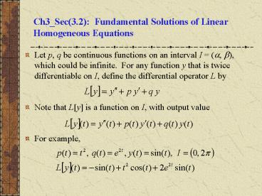
• Let p, q be continuous functions on an interval I
  (?, ?), which could be infinite. For any
  function y that is twice differentiable on I,
  define the differential operator L by
• Note that Ly is a function on I, with output
  value
• For example,

2
Differential Operator Notation

• In this section we will discuss the second order
  linear homogeneous equation Ly(t) 0, along
  with initial conditions as indicated below
• We would like to know if there are solutions to
  this initial value problem, and if so, are they
  unique.
• Also, we would like to know what can be said
  about the form and structure of solutions that
  might be helpful in finding solutions to
  particular problems.
• These questions are addressed in the theorems of
  this section.

3
Theorem 3.2.1 (Existence and Uniqueness)

• Consider the initial value problem
• where p, q, and g are continuous on an open
  interval I that contains t0. Then there exists a
  unique solution y ?(t) on I.
• Note While this theorem says that a solution to
  the initial value problem above exists, it is
  often not possible to write down a useful
  expression for the solution. This is a major
  difference between first and second order linear
  equations.

4
Example 1

• Consider the second order linear initial value
  problem
• Wrting the differential equation in the form
• The only points of discontinuity for these
  coefficients are t 0 and t 3. So the
  longest open interval containing the initial
  point t 1 in which all the coefficients are
  continuous is 0 lt t lt 3
• Therefore, the longest interval in which Theorem
  3.2.1 guarantees the existence of the solution is
  0 lt t lt 3

5
Example 2

• Consider the second order linear initial value
  problem
• where p, q are continuous on an open interval I
  containing t0.
• In light of the initial conditions, note that y
  0 is a solution to this homogeneous initial value
  problem.
• Since the hypotheses of Theorem 3.2.1 are
  satisfied, it follows that y 0 is the only
  solution of this problem.

6
Theorem 3.2.2 (Principle of Superposition)

• If y1and y2 are solutions to the equation
• then the linear combination c1y1 y2c2 is also
  a solution, for all constants c1 and c2.
• To prove this theorem, substitute c1y1 y2c2 in
  for y in the equation above, and use the fact
  that y1 and y2 are solutions.
• Thus for any two solutions y1 and y2, we can
  construct an infinite family of solutions, each
  of the form y c1y1 c2 y2.
• Can all solutions can be written this way, or do
  some solutions have a different form altogether?
  To answer this question, we use the Wronskian
  determinant.

7
The Wronskian Determinant (1 of 3)

• Suppose y1 and y2 are solutions to the equation
• From Theorem 3.2.2, we know that y c1y1 c2 y2
  is a solution to this equation.
• Next, find coefficients such that y c1y1 c2
  y2 satisfies the initial conditions
• To do so, we need to solve the following
  equations

8
The Wronskian Determinant (2 of 3)

• Solving the equations, we obtain
• In terms of determinants

9
The Wronskian Determinant (3 of 3)

• In order for these formulas to be valid, the
  determinant W in the denominator cannot be zero
• W is called the Wronskian determinant, or more
  simply, the Wronskian of the solutions y1and y2.
  We will sometimes use the notation

10
Theorem 3.2.3

• Suppose y1 and y2 are solutions to the equation
• with the initial conditions
• Then it is always possible to choose constants
  c1, c2 so that
• satisfies the differential equation and
  initial conditions if and ony if the Wronskian
• is not zero at the point t0

11
Example 3

• In Example 2 of Section 3.1, we found that
• were solutions to the differential equation
• The Wronskian of these two functions is
• Since W is nonzero for all values of t, the
  functions
• can be used to construct solutions of the
  differential equation with initial conditions at
  any value of t

12
Theorem 3.2.4 (Fundamental Solutions)

• Suppose y1 and y2 are solutions to the equation
• Then the family of solutions
• y c1y1 c2 y2
• with arbitrary coefficients c1, c2 includes
  every solution to the differential equation if an
  only if there is a point t0 such that
  W(y1,y2)(t0) ? 0, .
• The expression y c1y1 c2 y2 is called the
  general solution of the differential equation
  above, and in this case y1 and y2 are said to
  form a fundamental set of solutions to the
  differential equation.

13
Example 4

• Consider the general second order linear equation
  below, with the two solutions indicated
• Suppose the functions below are solutions to this
  equation
• The Wronskian of y1and y2 is
• Thus y1and y2 form a fundamental set of solutions
  to the equation, and can be used to construct all
  of its solutions.
• The general solution is

14
Example 5 Solutions (1 of 2)

• Consider the following differential equation
• Show that the functions below are fundamental
  solutions
• To show this, first substitute y1 into the
  equation
• Thus y1 is a indeed a solution of the
  differential equation.
• Similarly, y2 is also a solution

15
Example 5 Fundamental Solutions (2 of 2)

• Recall that
• To show that y1 and y2 form a fundamental set of
  solutions, we evaluate the Wronskian of y1 and
  y2
• Since W ? 0 for t gt 0, y1, y2 form a fundamental
  set of solutions for the differential equation

16
Theorem 3.2.5 Existence of Fundamental Set of
Solutions

• Consider the differential equation below, whose
  coefficients p and q are continuous on some open
  interval I
• Let t0 be a point in I, and y1 and y2 solutions
  of the equation with y1 satisfying initial
  conditions
• and y2 satisfying initial conditions
• Then y1, y2 form a fundamental set of solutions
  to the given differential equation.

17
Example 6 Apply Theorem 3.2.5 (1 of 3)

• Find the fundamental set specified by Theorem
  3.2.5 for the differential equation and initial
  point
• In Section 3.1, we found two solutions of this
  equation
• The Wronskian of these solutions is W(y1,
  y2)(t0) -2 ? 0 so they form a fundamental set
  of solutions.
• But these two solutions do not satisfy the
  initial conditions stated in Theorem 3.2.5, and
  thus they do not form the fundamental set of
  solutions mentioned in that theorem.
• Let y3 and y4 be the fundamental solutions of Thm
  3.2.5.

18
Example 6 General Solution (2 of 3)

• Since y1 and y2 form a fundamental set of
  solutions,
• Solving each equation, we obtain
• The Wronskian of y3 and y4 is
• Thus y3, y4 form the fundamental set of solutions
  indicated in Theorem 3.2.5, with general solution
  in this case

19
Example 6 Many Fundamental Solution Sets (3
of 3)

• Thus
• both form fundamental solution sets to the
  differential equation and initial point
• In general, a differential equation will have
  infinitely many different fundamental solution
  sets. Typically, we pick the one that is most
  convenient or useful.

20
Theorem 3.2.6

• Consider again the equation (2)
• where p and q are continuous real-valued
  functions. If y u(t) iv(t) is a
  complex-valued solution of Eq. (2), then its real
  part u and its imaginary part v are also
  solutions of this equation.

21
Theorem 3.2.6 (Abels Theorem)

• Suppose y1 and y2 are solutions to the equation
• where p and q are continuous on some open
  interval I. Then the W(y1,y2)(t) is given by
• where c is a constant that depends on y1 and y2
  but not on t.
• Note that W(y1,y2)(t) is either zero for all t in
  I (if c 0) or else is never zero in I (if c ?
  0).

22
Example 7 Apply Abels Theorem

• Recall the following differential equation and
  its solutions
• with solutions
• We computed the Wronskian for these solutions to
  be
• Writing the differential equation in the standard
  form
• So and the Wronskian given
  by Thm.3.2.6 is
• This is the Wronskian for any pair of fundamental
  solutions. For the solutions given above, we must
  let c -3/2

23
Summary

• To find a general solution of the differential
  equation
• we first find two solutions y1 and y2.
• Then make sure there is a point t0 in the
  interval such that W(y1, y2)(t0) ? 0.
• It follows that y1 and y2 form a fundamental set
  of solutions to the equation, with general
  solution y c1y1 c2 y2.
• If initial conditions are prescribed at a point
  t0 in the interval where W ? 0, then c1 and c2
  can be chosen to satisfy those conditions.