Linear Programming Problem

1
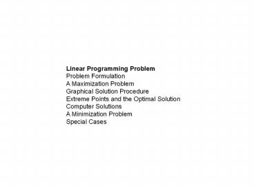
Linear Programming Problem Problem Formulation A
Maximization Problem Graphical Solution
Procedure Extreme Points and the Optimal
Solution Computer Solutions A Minimization
Problem Special Cases
2
The maximization or minimization of some quantity
is the objective in all linear programming
problems. All LP problems have constraints that
limit the degree to which the objective can be
pursued. A feasible solution satisfies all the
problem's constraints. An optimal solution is a
feasible solution that results in the largest
possible objective function value when maximizing
(or smallest when minimizing). A graphical
solution method can be used to solve a linear
program with two variables.
3
If both the objective function and the
constraints are linear, the problem is referred
to as a linear programming problem. Linear
functions are functions in which each variable
appears in a separate term raised to the first
power and is multiplied by a constant (which
could be 0). Linear constraints are linear
functions that are restricted to be "less than or
equal to", "equal to", or "greater than or equal
to" a constant.
4
Problem formulation or modeling is the process of
translating a verbal statement of a problem into
a mathematical statement.
5
Understand the problem thoroughly. Describe the
objective. Describe each constraint. Define the
decision variables. Write the objective in terms
of the decision variables. Write the constraints
in terms of the decision variables.
6
Example 1 LP Formulation
Max 5x1 7x2
s.t. x1 lt 6
2x1 3x2 lt
19
x1 x2 lt 8
x1, x2 gt 0
7

• - Prepare a graph of the feasible solutions for
  each of the constraints.
• - Determine the feasible region that satisfies
  all the constraints simultaneously.
• - Draw an objective function line.
• - Move parallel objective function lines toward
  larger objective function values without entirely
  leaving the feasible region.
• Any feasible solution on the objective function
  line with the largest value is an optimal
  solution.
• Verify that the optimal solution occurs at a
  vertex with coordinated X1 5, and X2 3.

8

• Constraint 2 Graphed

x2
(0, 6 1/3)
2x1 3x2 19
(9 1/2, 0)
x1
9
x2
8 7 6 5 4 3 2 1 1 2
3 4 5 6 7 8 9
10
Feasible Region
x1
10
x2
Objective Function 5x1 7x2 46
Optimal Solution (x1 5, x2 3)
x1
11
Slack and surplus variables represent the
difference between the left and right sides of
the constraints.
12
We see from your graph that Objective
Function Value 46 Decision Variable 1
(x1) 5 Decision Variable 2 (x2)
3 Slack in Constraint 1 1 ( 6
- 5) Slack in Constraint 2 0 (
19 - 19) Slack in Constraint 3 0
( 8 - 8)
13
Solve graphically for the optimal solution Max
2x1 6x2 s.t. 4x1 3x2 lt 12
2x1 x2 gt 8 x1, x2 gt
0 Conclusion Infeasible
14

• Solve graphically for the optimal solution
• Max 3x1 4x2
• s.t. x1 x2 gt 5
• 3x1 x2 gt 8
• x1, x2 gt 0
• Conclusion Unbounded

15
Solve Min 5x1 2x2 s.t. 2x1
5x2 gt 10 4x1 - x2 gt 12
x1 x2 gt 4 x1,
x2 gt 0
16
Min z 5x1 2x2 4x1 - x2 gt 12 x1 x2 gt
4
x2
5 4 3 2 1

2x1 5x2 gt 10
1 2 3 4 5
6
x1
17
Solve for the Extreme Point at the Intersection
of the Two Binding Constraints
4x1 - x2 12 x1 x2 4
Adding these two equations gives
5x1 16 or x1 16/5. Substituting
this into x1 x2 4 gives x2 4/5