
Molecular Evolution: Plan for week PowerPoint PPT Presentation
Title: Molecular Evolution: Plan for week
1
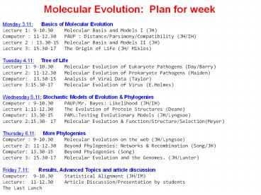
Molecular Evolution Plan for week
Monday 3.11 Basics of Molecular Evolution
Lecture 1 9-10.30 Molecular Basis and Models
I (JH) Computer 11-12.30 PAUP
Distance/Parsimony/Compatibility (JH/IH) Lecture
2 13.30-15 Molecular Basis and Models II
(JH) Lecture 3 15.30-17 The Origin of Life
(JH/ Miklos) Tuesday 4.11 Tree of Life
Lecture 1 9-10.30 Molecular Evolution of
Eukaryote Pathogens (Day/Barry) Lecture 2
11-12.30 Molecular Evolution of Prokaryote
Pathogens (Maiden) Computer 13.30-15 Analysis
of Viral Data (Taylor) Lecture 315.30-17
Molecular Evolution of Virus (E.Holmes)
Wednesday 5.11 Stochastic Models of Evolution
Phylogenies Computer 9-10.30 PAUP/Mr.
Bayes Likelihood (JH/IH) Lecture 111-12.30
The Evolution of Protein Structures
(Deane) Computer 13.30-15 PAMLTesting
Evolutionary Models (JH/Lyngsoe) Lecture 215.30-
17 Molecular Evolution Function/Structure/Sele
ction(Meyer) Thursday 6.11 More
Phylogenies Computer 9-10.30 Molecular
Evolution on the web (JH/Lyngsoe) Lecture 2
11-12.30 Beyond Phylogenies Networks
Recombination (Song/JH) Computer 13.30-15
Beyond Phylogenies (Song) Lecture 3 15.30-17
Molecular Evolution and the Genomes.
(JH/Lunter) Friday 7.11 Results, Advanced
Topics and article discussion Computer 9-10.30
Statistical Alignment (JH/IM) Lecture
11-12.30 Article Discussion/Presentation by
students The Last Lunch
2
Two Discussion Articles
1. Timing the ancestor of the HIV-1 pandemic
strains.Korber B, Muldoon M, Theiler J, Gao F,
Gupta R, Lapedes A, Hahn BH, Wolinsky S,
Bhattacharya T. Science. 2000 Jun
9288(5472)1789-96.
2. Sequencing and comparison of yeast species
to identify genes and regulatory elements.
Kells, M., N.Patterson, M.Endrizzi E.Lander
Nature May 15 2003 vol 423.241-
3
The Data its growth.
- 1976/79 The first viral genome MS2/fX174
- 1995 The first prokaryotic genome H.
influenzae - 1996 The first unicellular eukaryotic genome
- Yeast - 1997 The first multicellular eukaryotic
genome C.elegans - The human genome
- The Mouse Genome
1.5.03 Known gt1000 viral genomes 96
prokaryotic genomes 16 Archeobacterial
genomes A series multicellular genomes are coming.
A general increase in data involving higher
structures and dynamics of biological systems
4
The Nucleotides
Transversions
Purines
Pyremidines
Transitions
http//www.accessexcellence.org/AB/GG/
5
The Amino Acids/Codons/Genes
nucleotides3 ? amino acids, stop
http//www.accessexcellence.org/AB/GG/
6
Major Application Areas of Molecular Evolution
Phylogenies and Classification Rates of Evolution
The Molecular Clock Dating Functional
Constraint Negative Selection. Positive/Diversif
ying Selection Structure RNA Structure Gene
Finding Homing in on Important Genes Homology
Searches Disease Gene Mapping
7
The Tree (?) of Life
Plant
Fungi
Animals
8
Tree of Life.
Science vol.300 June 2003
9
The Origin of Life
When did life originate? Is the present structure
a necessity or is it random accident? How
frequent is life in the Universe?
-
Self replication easy Self assembly easy Many
extrasolar planets
Hard to make proper polymerisation No convincing
scenario. No testability
Increased Origin Research In preparation of
future NASA expeditions. The rise of nano
biology. The ability to simulate larger
molecular systems
10
Central Principles of Phylogeny Reconstruction
TTCAGT TCCAGT GCCAAT GCCAAT
1
0
2
Parsimony Distance Likelihood
Total Weight 4
0
1
0.6
1 1 2 3 2 1
0.7
1.5
0.4
0.3
L3.110-7 Parameter estimates
11
From Distance to Phylogenies
What is the relationship of a, b, c, d e?
Molecular clock
A b c d
e A - 22 10 22
22 B 6 - 22 16
14 C 7 3 - 22
22 D 13 9 8 -
16 e 6 8 9
15 -
No Molecular clock
12
Enumerating Trees Unrooted valency 3
Recursion Tn (2n-5) Tn-1
Initialisation T1 T2 T31
4 5 6 7 8 9 10 15 20
3 15 105 945 10345 1.4 105 2.0 106 7.9 1012 2.2 1020
13
Heuristic Searches in Tree Space
Nearest Neighbour Interchange
T1
T1
T3
T1
T2
T3
T3
T4
T4
T2
T2
T4
Subtree regrafting
s4
s6
s1
s4
s6
T4
s2
s5
s5
s3
s3
s1
T3
T3
T4
s2
Subtree rerooting and regrafting
s4
s6
s1
s4
s6
T4
s2
s5
s5
s3
s1
s3
T3
T3
T4
s2
14
Assignment to internal nodes The simple way.
A
G
C
T
?
?
?
?
?
?
C
C
C
A
What is the cheapest assignment of nucleotides to
internal nodes, given some (symmetric) distance
function d(N1,N2)??
If there are k leaves, there are k-2 internal
nodes and 4k-2 possible assignments of
nucleotides. For k22, this is more than 1012.
15
5S RNA Alignment Phylogeny Hein, 1990
3
5
4
6
13
11
9
7
15
17
14
10
12
16
Transitions 2, transversions 5 Total weight
843.
8
2
1
10 tatt-ctggtgtcccaggcgtagaggaaccacaccgatccatctcga
acttggtggtgaaactctgccgcggt--aaccaatact-cg-gg-ggggg
ccct-gcggaaaaatagctcgatgccagga--ta 17
t--t-ctggtgtcccaggcgtagaggaaccacaccaatccatcccgaact
tggtggtgaaactctgctgcggt--ga-cgatact-tg-gg-gggagccc
g-atggaaaaatagctcgatgccagga--t- 9
t--t-ctggtgtctcaggcgtggaggaaccacaccaatccatcccgaact
tggtggtgaaactctattgcggt--ga-cgatactgta-gg-ggaagccc
g-atggaaaaatagctcgacgccagga--t- 14
t----ctggtggccatggcgtagaggaaacaccccatcccataccgaact
cggcagttaagctctgctgcgcc--ga-tggtact-tg-gg-gggagccc
g-ctgggaaaataggacgctgccag-a--t- 3
t----ctggtgatgatggcggaggggacacacccgttcccataccgaaca
cggccgttaagccctccagcgcc--aa-tggtact-tgctc-cgcaggga
g-ccgggagagtaggacgtcgccag-g--c- 11
t----ctggtggcgatggcgaagaggacacacccgttcccataccgaaca
cggcagttaagctctccagcgcc--ga-tggtact-tg-gg-ggcagtcc
g-ctgggagagtaggacgctgccag-g--c- 4
t----ctggtggcgatagcgagaaggtcacacccgttcccataccgaaca
cggaagttaagcttctcagcgcc--ga-tggtagt-ta-gg-ggctgtcc
c-ctgtgagagtaggacgctgccag-g--c- 15
g----cctgcggccatagcaccgtgaaagcaccccatcccat-ccgaact
cggcagttaagcacggttgcgcccaga-tagtact-tg-ggtgggagacc
gcctgggaaacctggatgctgcaag-c--t- 8
g----cctacggccatcccaccctggtaacgcccgatctcgt-ctgatct
cggaagctaagcagggtcgggcctggt-tagtact-tg-gatgggagacc
tcctgggaataccgggtgctgtagg-ct-t- 12
g----cctacggccataccaccctgaaagcaccccatcccgt-ccgatct
gggaagttaagcagggttgagcccagt-tagtact-tg-gatgggagacc
gcctgggaatcctgggtgctgtagg-c--t- 7
g----cttacgaccatatcacgttgaatgcacgccatcccgt-ccgatct
ggcaagttaagcaacgttgagtccagt-tagtact-tg-gatcggagacg
gcctgggaatcctggatgttgtaag-c--t- 16
g----cctacggccatagcaccctgaaagcaccccatcccgt-ccgatct
gggaagttaagcagggttgcgcccagt-tagtact-tg-ggtgggagacc
gcctgggaatcctgggtgctgtagg-c--t- 1
a----tccacggccataggactctgaaagcactgcatcccgt-ccgatct
gcaaagttaaccagagtaccgcccagt-tagtacc-ac-ggtgggggacc
acgcgggaatcctgggtgctgt-gg-t--t- 18
a----tccacggccataggactctgaaagcaccgcatcccgt-ccgatct
gcgaagttaaacagagtaccgcccagt-tagtacc-ac-ggtgggggacc
acatgggaatcctgggtgctgt-gg-t--t- 2
a----tccacggccataggactgtgaaagcaccgcatcccgt-ctgatct
gcgcagttaaacacagtgccgcctagt-tagtacc-at-ggtgggggacc
acatgggaatcctgggtgctgt-gg-t--t- 5
g---tggtgcggtcataccagcgctaatgcaccggatcccat-cagaact
ccgcagttaagcgcgcttgggccagaa-cagtact-gg-gatgggtgacc
tcccgggaagtcctggtgccgcacc-c--c- 13
g----ggtgcggtcataccagcgttaatgcaccggatcccat-cagaact
ccgcagttaagcgcgcttgggccagcc-tagtact-ag-gatgggtgacc
tcctgggaagtcctgatgctgcacc-c--t- 6
g----ggtgcgatcataccagcgttaatgcaccggatcccat-cagaact
ccgcagttaagcgcgcttgggttggag-tagtact-ag-gatgggtgacc
tcctgggaagtcctaatattgcacc-c-tt-
16
Cost of a history - minimizing over internal
states
A C G T
d(C,G) wC(left subtree)
A C G T
A C G T
17
Cost of a history leaves (initialisation).
A C G T
Initialisation leaves Cost(N) 0 if N is
at leaf, otherwise infinity
G
A
Empty Cost 0
Empty Cost 0
18
Fitch-Hartigan-Sankoff Algorithm
(A,C,G,T) (9,7,7,7)
(A, C, G,T) (10,2,10,2)
The cost of cheapest tree hanging from this node
given there is a C at this node
(A,C,G,T) 0
(A,C,G,T) 0
(A,C,G,T) 0
5
C
A
2
T
G
19
The Felsenstein Zone Felsenstein-Cavendar (1979)
True Tree
Reconstructed Tree
s1
s2
s3
s4
Patterns(16 only 8 shown) 0 1 0 0 0
0 0 0 0 0 1 0 0 1 0 1 0 0 0 1
0 1 1 0 0 0 0 0 1 0 1 1
20
Bootstrapping Felsenstein (1985)
ATCTGTAGTCT ATCTGTAGTCT ATCTGTAGTCT ATCTGTAGTCT 10
230101201
1
500
2
ATCTGTAGTCT ATCTGTAGTCT ATCTGTAGTCT ATCTGTAGTCT
?????????? ?????????? ?????????? ??????????
?????????? ?????????? ?????????? ??????????
2
3
2
3
2
3
4
4
1
1
4
1
21
The Molecular Clock
First noted by Zuckerkandl Pauling (1964) as an
empirical fact. How can one detect it?
Known Ancestor, a, at Time t
22
Rootings
Purpose 1) To give time direction in the
phylogeny most ancient point 2) To be able to
define concepts such a monophyletic group.
1) Outgrup Enhance data set with sequence from
a species definitely distant to all of them. It
will be be joined at the root of the original data
2) Midpoint Find midpoint of longest path in
tree.
3) Assume Molecular Clock.
23
Rooting the 3 kingdoms
3 billion years ago no reliable clock - no
outgroup Given 2 set of homologous proteins, i.e.
MDH LDH can the archea, prokaria and eukaria be
rooted?
P
P
E
E
E
Root??
MDH
LDH
P
A
A
A
Given 2 set of homologous proteins, i.e. MDH
LDH can the archea, prokaria and eukaria be
rooted?
LDH/MDH
LDH/MDH
E
P
A
E
P
A
24
Non-contemporaneous leaves. (A.Rambaut (2000)
Estimating the rate of molecular evolution
incorporating non-contemporaneous sequences into
maximum likelihood phylogenies. Bioinformatics
16.4.395-399)
time
Contemporary sample no time structure
Serial sample with time structure
1980
1990
2000
RNA viruses like HIV evolve fast enough that you
cant ignore the time structure
From Drummond
25
HIV-1 (env) evolution in nine infected individuals
Shankarappa et al (1999)
From Drummond
26
A tree sampled from the posterior distribution of
Shankarappa Patient
Ladder-like appearance
Lineage A
Lineage B
- 210 sequences collected over a period of 9.5
years - 660 nucleotides from env C2-V5 region
- Only first 285 (no alignment ambiguities) were
used in this analysis - Effective population size and mutation rate were
co-estimated using Bayesian MCMC.
Ne 4000,6300 Mu 0.8 1 per site year
From Drummond
27
Models of Amino Acid, Nucleotide Codon Evolution
Amino Acids, Nucleotides Codons Continuous
Time Markov Processes Specific Models Special
Issues Context Dependence Rate Variation
28
The Purpose of Stochastic Models.
- Molecular Evolution is Stochastic.
- 2. To estimate evolutionary parameters, not
observable directly - i. Real number of events in evolutionary
history. - ii. Rates of different kinds of events in
evolutionary history. - iii. Strength of selection against amino acid
changing nucleotide substitutions. - iv. Estimate importance of different
biological factors. - Survive a goodness of fit test.
- 4. Serve these purposes as simply as possible.
29
Central Problems History cannot be observed,
only end products.
ACGTC
ACGTC
ACGCC
ACGCC
AGGCC
AGGCC
AGGCT
AGGCT
AGGGC
AGGCT
AGGCT
AGGTT
AGGTT
AGTGC
Comment Even if History could be observed, the
underlying process couldnt
30
Principle of Inference Likelihood
Likelihood function L() the probability of data
as function of parameters L(Q,D) LogLikelihood
Function l() ln(L(Q,D))
If the data is a series of independent
experiments L() will become a product of
Likelihoods of each experiment, l() will become
the sum of LogLikelihoods of each experiment
In Likelihood analysis parameter is not viewed as
a random variable.
31
Likelihood and logLikelihood of Coin Tossing
From Edwards (1991) Likelihood
32
Principle of Inference Bayesian Analysis
In Bayesian Analysis the parameters are viewed as
stochastic variables that has a prior
distribution before observing data. Data depend
on the parameters and after observing the data,
the parameters will have a posterior distribution.
33
Simplifying Assumptions I
Data s1TCGGTA,s2TGGTT
Probability of Data
Biological setup
a - unknown
1) Only substitutions. s1 TCGGTA s1
TCGGA s2 TGGT-T
s2 TGGTT
2) Processes in different positions of the
molecule are independent, so the probability for
the whole alignment will be the product of the
probabilities of the individual patterns.
a5
a4
a3
a2
a1
T
A
T
G
G
G
G
C
T
T
34
Simplifying Assumptions II
3) The evolutionary process is the same in all
positions
4) Time reversibility Virtually all models of
sequence evolution are time reversible. I.e. pi
Pi,j(t) pj Pj,i(t), where pi is the stationary
distribution of i and Pt(i-gtj) the probability
that state i has changed into state j after t
time. This implies that
Pa,N1(l1)Pa,N2(l2)
PN1,N2(l1l2)
a
l2l1
l1
l2
N2
N1
N2
N1
35
Simplifying assumptions III
5) The nucleotide at any position evolves
following a continuous time Markov Chain.
Pi,j(t) continuous time markov chain on the state
space A,C,G,T.
t1
e
A
t2
C
C
Q - rate matrix
T O
A C G
T F A -(qA,CqA,GqA,T) qA,C
qA,G qA,T R C qC,A
-(qC,AqC,GqC,T) qC, G qC
,T O G qG,A qG,C
-(qG,AqG,CqG,T) qG,T M T qT,A
qT,C qT,G
-(qT,AqT,CqT,G)
6) The rate matrix, Q, for the continuous time
Markov Chain is the same at all times (and often
all positions). However, it is possible to let
the rate of events, ri, vary from site to site,
then the term for passed time, t, will be
substituted by rit.
36
Q and P(t)
What is the probability of going from i (C?) to j
(G?) in time t with rate matrix Q?
i. P(0) I. ii. P(e) close to IeQ
for e small. iii. P'(0) Q. iv.
lim P(t) has the equilibrium frequencies of the 4
nucleotides in each row. v. Waiting time in
state j, Tj, P(Tj gt t) e -(qjjt) vi. QE0
Eij1 (all i,j) vii. PEE
viii If ABBA, then eABeAeB.
37
Jukes-Cantor 69 Total Symmetry
Rate-matrix, R
T O
A C
G T F
A -3a a
a a R C
a -3a
a a O G a
a -3 a
a M T a
a a
-3 a Transition prob. after time t, a
at P(equal) ¼(1 3e-4a ) 1 - 3a
P(diff.) ¼(1 - 3e-4a )
3a Stationary Distribution (1,1,1,1)/4.
38
Geometric/Exponential Distributions The
Geometric Distribution 0,1,.. Geo(p)
PZj)pj(1-p) PZgtj)pj E(Z)1/p. The
Exponential Distribution R Exp(a)
Density f(t) ae-at, P(Xgtt) e-at
Mean 2.5
Properties X Exp(a) Y Exp(b) independent
i. P(Xgtt2Xgtt1) P(Xgtt2-t1) (t2 gt t1)
Markov (memoryless) process ii. E(X)
1/a. iii. P(Zgtt)()P(Xgtt) small a
(pe-a). iv. P(X lt Y) a/(a b). v.
min(X,Y) Exp (a b).
N
39
Comparison of Pairs of Nucleotides/Sequences
Shortest Path
Sample Paths according to their probability
All Evolutionary Paths
All Evolutionary Paths
C
CTACGT
C
C
G
G
G
GTATAT
ATTGTGTATATAT.CAG ATTGCGTATCTAT.CCG
Chimp
Mouse
E.coli
Higher Cells
Fish
40
From Q to P for Jukes-Cantor
41
Kimura 2-parameter model
TO A
C
G T F
A -2b-a b
a
b R C
b -2b-a
b
a O G a
b
-2b-a b M T
b a
b
-2b-a a at b
bt
Q
P(t)
42
Felsenstein81 Hasegawa, Kishino Yano 85
Unequal base composition (Felsenstein,
1981) Qi,j Cpj i unequal j
Transition/transversion compostion bias
(Hasegawa, Kishino Yano, 1985)
(a/b)Cpj i- gtj a transition Qi,j
Cpj i- gtj a
transversion
43
Dayhoffs empirical approach (1970)
Take a set of closely related proteins, count all
differences and make symmetric difference matrix,
since time direction cannot be observed.
If qijqji, then equilibrium frequencies, pi, are
all the same.
The transformation qij --gt piqij/pj, then
equilibrium frequencies will be pi.
44
Measuring Selection
ThrSer ACGTCA
ThrPro ACGCCA
Certain events have functional consequences and
will be selected out. The strength and
localization of this selection is of great
interest.
ThrSer ACGCCG
ArgSer AGGCCG
The selection criteria could in principle be
anything, but the selection against amino acid
changes is without comparison the most important
ThrSer ACTCTG
AlaSer GCTCTG
AlaSer GCACTG
I
45
The Genetic Code
3 classes of sites 4 2-2 1-1-1-1
4 (3rd)
1-1-1-1 (3rd)
ii. T?A (2nd)
Problems i. Not all fit into those
categories. ii. Change in on site can change the
status of another.
46
Possible events if the genetic code remade from
Li,1997
Possible number of substitutions 61 (codons)3
(positions)3 (alternative nucleotides).
Substitutions Number
Percent Total in all codons 549
100 Synonymous
134 25 Nonsynonymous
415 75
Missense 392
71 Nonsense 23
4
N
47
Synonyous (silent) Non-synonymous (replacement)
substitutions
Ser Thr Glu Met Cys Leu Met Gly Thr
TCA ACT GAG ATG TGT TTA ATG GGG ACG
GGG ACA GGG ATA TAT CTA ATG GGT AGC Ser
Thr Gly Ile Tyr Leu Met Gly Ser Ks Number of
Silent Events in Common History Ka Number of
Replacement Events in Common History Ns Silent
positions Na replacement positions. Rates per
pos ((Ks/Ns)/2T) Example Ks 100 Ns 300
T108 years Silent rate (100/300)/2108 1.66
10-9 /year/pos.
Thr ACC
Thr ACG
Ser AGC
Miyata use most silent path for calculations.
Arg AGG
48
Kimuras 2 parameter model Lis Model.
Probabilities
Rates
start
Selection on the 3 kinds of sites
(a,b)?(?,?) 1-1-1-1
(fa,fb) 2-2
(a,fb) 4 (a, b)
49
alpha-globin from rabbit and mouse.
Ser Thr Glu Met Cys Leu Met Gly Gly TCA ACT GAG
ATG TGT TTA ATG GGG GGA
TCG ACA GGG ATA TAT CTA ATG GGT ATA Ser
Thr Gly Ile Tyr Leu Met Gly Ile
- Sites Total Conserved
Transitions Transversions - 1-1-1-1 274 246 (.8978)
12(.0438) 16(.0584) - 2-2 77 51 (.6623)
21(.2727) 5(.0649) - 4 78 47 (.6026)
16(.2051) 15(.1923) - Z(at,bt) .501exp(-2at) - 2exp(-t(ab)
transition Y(at,bt) .251-exp(-2bt )
(transversion) - X(at,bt) .251exp(-2at) 2exp(-t(ab)
identity - L(observations,a,b,f)
- C(429,274,77,78) X(af,bf)246Y(af,bf)12Z(a
f,bf)16 X(a,bf)51Y(a,bf)21Z(a,bf)5X(a,
b)47Y(a,b)16Z(a,b)15 - where a at and b bt.
- Estimated Parameters a 0.3003 b
0.1871 2b 0.3742 (a 2b) 0.6745 f
0.1663 - Transitions
Transversions - 1-1-1-1 af 0.0500 2bf 0.0622
- 2-2 a 0.3004 2bf 0.0622
- 4 a 0.3004 2b 0.3741
50
HIV2 Analysis
Hasegawa, Kisino Yano Subsitution Model
Parameters at ßt pA
pC pG pT 0.350 0.105
0.361 0.181 0.236 0.222 0.015
0.005 0.004 0.003 0.003 Selection
Factors GAG 0.385 (s.d. 0.030) POL 0.220 (s.
d. 0.017) VIF 0.407 (s.d. 0.035) VPR 0.494 (
s.d. 0.044) TAT 1.229 (s.d.
0.104) REV 0.596 (s.d. 0.052) VPU 0.902 (s.d.
0.079) ENV 0.889 (s.d. 0.051) NEF 0.928 (s.
d. 0.073) Estimated Distance per Site 0.194
51
Examples of rates remade from Li,1997
Organism Gene Syno/year
Non-Syno/Year
RNA Virus Influenza A Hemagglutinin 13.1
10-3 3.6 10-3 Hepatitis C E
6.9 10-3 0.3 10-3 HIV 1
gag 2.8 10-3 1.7
10-3 DNA virus Hepatitis B P
4.6 10-5 1.5 10-5 Herpes Simplex
Genome 3.5 10-8 Nuclear Genes Mammals
c-mos 5.2 10-9 0.9
10-9 Mammals a-globin 3.9 10-9
0.6 10-9 Mammals histone 3
6.2 10-9 0.0
N
52
Codon based Models Goldman,Yang Muse,Gaut
- Codons as the basic unit.
- ii. A codon based matrix would have (6161)-61 (
3661) off-diagonal entries. - i. Bias in nucleotide usage.
- ii. Bias in codon usage.
- iii. Bias in amino acid usage.
- iv. Synonymous/non-synonymous distinction.
- v. Amino acid distance.
- vi. Transition/transversion bias.
- codon i and codon j differing by one
nucleotide, then - apj exp(-di,j/V) differs by
transition - qi,j
- bpj exp(-di,j/V) differs by
transversion. - -di,j is a physico-chemical difference between
amino acid i and amino acid j. V is a factor
that reflects the variability of the gene
involved.
53
Rate variation between sitesiid each site
- The rate at each position is drawn independently
from a distribution, typically a G (or lognormal)
distribution. G(a,b) has density xb-1e-ax/G(b)
, where a is called scale parameter and b form
parameter. - Let L(pi,Q,t) be the likelihood for observing
the i'th pattern, t all time lengths, Q the
parameters describing the process parameters and
f (ri) the continuous distribution of rate(s).
Then
54
Rate variation between sitesiid Hidden Markov
Chains
- Different positions in the molecule evolves at
different rates. For instance fast or slow rF or
slow rS. - 2) The rates at neighbor positions evolve at the
same rate.
O1 O2 O3 O4 O5 O6 O7 O8 O9
O10
F
S
What is the probability of the data? What is the
most probable hidden configuration? What is the
probability of specific hidden state?
55
Statistical Test of Models (Goldman,1990)
Data 3 sequences of length L ACGTTGCAA
... AGCTTTTGA ... TCGTTTCGA ...
A. Likelihood (free multinominal model 63 free
parameters) L1 pAAAAAA...pAACAAC...pTTTTTT
where pN1N2N3 (N1N2N3)/L
B. Jukes-Cantor and unknown branch lengths
L2 pAAA(l1',l2',l3') AAA...pTTT(l1',l2',l3')
TTT
Test statistics I. (expected-observed)2/exp
ected or II -2 lnQ 2(lnL1 - lnL2) JC69
Jukes-Cantor 3 parameters gt c2 60 d.of
freedom Problems i. To few observations pr.
pattern. ii. Many competing
hypothesis. Parametric bootstrap i. Maximum
likelihood to estimate the parameters.
ii. Simulate with estimated model. iii. Make
simulated distribution of -2 lnQ.
iv. Where is real -2 lnQ in this
distribution?
56
Episodic Evolution
Poisson Process i. Ti's independent,
exponentially distributed with same parameter
(l). ii. Variance and Mean both l.
Emperical Observations i. Variance/Mean gt 1
(clumpy process) for non-synonymous event
Possible explanations i. Selective
Avalances. ii. Gene conversions from pseudogenes.
57
Assignment to internal nodes The simple way.
A
G
C
T
?
?
?
?
?
?
C
C
C
A
If branch lengths and evolutionary process is
known, what is the probability of nucleotides at
the leaves?
Cctacggccatacca a ccctgaaagcaccccatcccgt
Cttacgaccatatca c cgttgaatgcacgccatcccgt
Cctacggccatagca c ccctgaaagcaccccatcccgt
Cccacggccatagga c ctctgaaagcactgcatcccgt
Tccacggccatagga a ctctgaaagcaccgcatcccgt
Ttccacggccatagg c actgtgaaagcaccgcatcccg Tggt
gcggtcatacc g agcgctaatgcaccggatccca
Ggtgcggtcatacca t gcgttaatgcaccggatcccat
58
Probability of leaf observations - summing over
internal states
A C G T
P(C?G) PC(left subtree)
A C G T
A C G T
59
Output from Likelihood Method.
Molecular Clock
No Molecular Clock
s3
s4
23 -/5.2
10.9 -/2.1
s1
11.6 -/2.1
3.9 -/0.8
Duplication Times
9.9 -/1.2
Amount of Evolution
12 -/2.2
4.1 -/0.7
11.1 -/1.8
11.4 -/1.9
6.9 -/1.3
5.9 -/1.2
s2
s5
Now
s5
s1
s2
s3
s4
2n-3 lengths estimated
n-1 heights estimated
Likelihood 7.910-14 ?? ? 0.31 0.18
Likelihood 6.210-12 ?? ? 0.34 0.16
ln(7.910-14) ln(6.210-12) is ?2 distributed
with (n-2) degrees of freedom
60
The generation/year-time clock Langley-Fitch,1973
Absolute Time Clock
s2
l2
l1 l2 lt l3
l1
s1
l3
Some rooting techniquee
l3
l1 l2
s3
s2
s1
s3
Generation Time Clock
100 Myr
constant
Generation Time
variable
Absolute Time Clock
Elephant
Mouse
61
The generation/year-time clock Langley-Fitch,1973
Generation Time Clock
Any Tree
Can the generation time clock be tested?
s2
s1
s3
Assume, a data set 3 species, 2 sequences each
s2
s1
s3
s2
s1
s2
s1
s3
s3
62
The generation/year-time clock Langley-Fitch,1973
s2
l2
l3
l1
s1
l3
l1 l2
s2
s1
s3
s3
dg 2
k3 degrees of freedom 3
dg k-1
k dg 2k-3
s2
cl2
s2
l2
cl1
l1
s1
s1
l3
cl3
s3
s3
k3, t2 dg4 k, t dg (2k-3)-(t-1)
63
- b globin, cytochrome c, fibrinopeptide A
generation time clock - Langley-Fitch,1973
Fibrinopeptide A phylogeny
- Relative rates
- a-globin 0.342
- globin 0.452
- cytochrome c 0.069
- fibrinopeptide A 0.137
Rat
Pig
Dog
Cow
Goat
Human
Horse
Rabbit
Gibbon
Monkey
Llama
Sheep
Donkey
Gorilla
N
64
Almost Clocks (MJ Sanderson (1997) A
Nonparametric Approach to Estimating Divergence
Times in the Absence of Rate Constancy
Mol.Biol.Evol.14.12.1218-31), J.L.Thorne et al.
(1998) Estimating the Rate of Evolution of the
Rate of Evolution. Mol.Biol.Evol.
15(12).1647-57, JP Huelsenbeck et al. (2000) A
compound Poisson Process for Relaxing the
Molecular Clock Genetics 154.1879-92. )
I Smoothing a non-clock tree onto a clock tree
(Sanderson). II Rate of Evolution of the rate
of Evolution (Thorne et al.). The rate of
evolution can change at each bifurcation. III
Relaxed Molecular Clock (Huelsenbeck et al.).
At random points in time, the rate changes by
multiplying with random variable (gamma
distributed)
Comment Makes perfect sense. Testing no clock
versus perfect is choosing between two
unrealistic extremes.
65
Summary
Phylogeny Principles of Phylogenies Rates of
Molecular Rates and the Molecular Clock Rooting
Phylogenies The Generation Time Clock Almost
Clocks Non-Contemporaneous Leaves (Viruses
Ancient DNA) The Purpose of Stochastic Models The
assumptions of Stochastic Models The Central
Models Measuring Selection Variation among
sites Testing Models.
66
History of Phylogenetic Methods Stochastic
Models 1958 Sokal and Michener publishes UGPMA
method for making distrance trees with a
clock. 1964 Parsimony principle defined, but not
advocated by Edwards and Cavalli-Sforza. 1962-65
Zuckerkandl and Pauling introduces the notion of
a Molecular Clock. 1967 First large molecular
phylogenies by Fitch and Margoliash. 1969
Heuristic method used by Dayhoff to make trees
and reconstruct ancetral sequences. 1969
Jukes-Cantor proposes simple model for amino acid
evolution. 1970 Neyman analyzes three sequence
stochastic model with Jukes-Cantor
substitution. 1971-73 Fitch, Hartigan Sankoff
independently comes up with same algorithm
reconstructing parsimony ancetral sequences.
1973 Sankoff treats alignment and phylogenies
as on general problem phylogenetic
alignment. 1979 Cavender and Felsenstein
independently comes up with same evolutionary
model where parsimony is inconsistent. Later
called the Felsenstein Zone. 1979 Kimura
introduces transition/transversion bias in
nucleotide model in response to pbulication of
mitochondria sequences. 1981 Felsenstein
Maximum Likelihood Model Program DNAML (i
programpakken PHYLIP). Simple nucleotide model
with equilibrium bias.
67
1981 Parsimony tree problem is shown to be
NP-Complete. 1985 Felsenstein introduces
bootstrapping as confidence interval on
phylogenies. 1985 Hasegawa, Kishino and Yano
combines transition/transversion bias with
unequal equilibrium frequencies. 1986 Bandelt
and Dress introduces split decomposition as a
generalization of trees. 1985- Many authors
(Sawyer, Hein, Stephens, M.Smith) tries to
address the problem of recombinations in
phylogenies. 1991 Gillespies book proposes
lumpy evolution. 1994 Goldman Yang Muse
Gaut introduces codon based models 1997-9 Thorne
et al., Sanderson Huelsenbeck introduces the
Almost Clock. 2000 Rambaut (and others) makes
methods that can find trees with
non-contemporaneous leaves. 2000 Complex Context
Dependent Models by Jensen Pedersen.
Dinucleotide and overlapping reading frames.
2001- Major rise in the interest in
phylogenetic statistical alignment 2001-
Comparative genomics underlines the functional
importance of molecular evolution.
68
References Books Journals
Joseph Felsenstein "Inferring Phylogenies 660
pages Sinauer 2003 Excellent focus on
methods and conceptual issues. Masatoshi Nei,
Sudhir Kumar Molecular Evolution and
Phylogenetics 336 pages Oxford University Press
Inc, USA 2000 R.D.M. Page, E. Holmes Molecular
Evolution A Phylogenetic Approach 352 pages
1998 Blackwell Science (UK) Dan Graur, Li
Wen-Hsiung Fundamentals of Molecular Evolution
Sinauer Associates Incorporated 439 pages
1999 Margulis, L and K.V. Schwartz (1998) Five
Kingdoms 500 pages Freeman A grand illustrated
tour of the tree of life Semple, C and M. Steel
Phylogenetics 2002 230 pages Oxford University
Press Very mathematical
Journals Journal of Molecular Evolution
http//www.nslij-genetics.org/j/jme.html Molecular
Biology and Evolution http//mbe.oupjournals.o
rg/ Molecular Phylogenetics and Evolution
http//www.elsevier.com/locate/issn/1055-7903 Syst
ematic Biology - http//systbiol.org/ J. of
Classification - http//www.pitt.edu/csna/joc.ht
ml
69
References www-pages
Tree of Life on the WWW http//tolweb.org/tree/phy
logeny.html http//www.treebase.org/treebase/
Software http//evolution.genetics.washington.edu/
phylip.html http//paup.csit.fsu.edu/ http//morph
bank.ebc.uu.se/mrbayes/ http//evolve.zoo.ox.ac.uk
/beast/ http//abacus.gene.ucl.ac.uk/software/paml
.html
Data Genome Centres http//www.ncbi.nih.gov/Entr
ez/ http//www.sanger.ac.uk
70
Next
Classification of Viruses Overhead with
considerations model?gt data. Example HMM
variation in rates, gamma rates. Example Almost
clock Example Episodic clock Example
Bootstrapping.
Recommended
