
Deep Subsurface Microbiology - PowerPoint PPT Presentation
1 / 70
Title: Deep Subsurface Microbiology
1
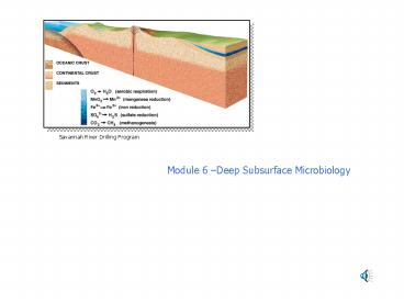
Deep Subsurface Microbiology
Savannah River Drilling Program
Module 6 Deep Subsurface Microbiology
2
Deep Subsurface Microbiology
Deep Subsurface Microbiology
- Deep aquifers (hundreds or thousands of metres
below surface) have only recently been
investigated other than by petroleum or sulfur
companies seeking deposits or concerned with the
impact of microorganisms on their drilling and
mining activities. - The first major project to investigate the deep
subsurface was started in 1986 at the U.S.
Department of Energy site at Savannah River. The
drilling, for the first time, was carried out
with microbial sampling as a prime objective.
Great care was taken to maintain the drill holes
in a state suitable for microbial sampling. - The Savannah River plant overlies the Atlantic
Coastal Plain and has unconsolidated sediments to
a depth of 300 metres. The sediments are then
underlain by crystalline metamorphic rock or
consolidated mudstone. There are some sandy
aquifers interspersed between the clay and silt
formations. - A sample drill hole was bored first to determine
the stratigraphy of the site. Then a sampling
hole was drilled. The drilling fluid (sodium
bentonite) was used to continuously flush the
hole as it was drilled. To prevent contamination,
the sampling container was lowered to a depth
below the circulating drilling fluid. Autoclaved
or steamed stainless steel core liners were used
to collect the samples. - The sediments were removed from the core liners
in a N2-flushed glove bag to preserve anaerobic
conditions. All transfers were done within 30
min. of sampling the drill hole.
3
Subsurface Environments
SLIMES, or subsurface lithoautotrophic microbial
ecosystems, exist in the pores between
interlocking mineral grains of many igneous
rocks. Autotrophic microbes (green) derive
nutrients and energy from inorganic chemicals in
their surroundings, and many other microbes
(red), in turn, feed on organics created by
autotrophs.
SUBSURFACE ENVIRONMENTS vary considerably in
the composition of the surrounding rock.
Deep-living microbes pervade both oceanic and
continental crust and are especially abundant in
sedimentary formations. Such microorganisms fail
to survive only where the temperature exceeds
about 110 degrees Celsius (orange areas). The
nature of the population does, however, change
from place to place. For example, a porous
sedimentary layer that acts as a conduit for
groundwater may contain both oxygen-rich (light
blue) and oxygen-poor (dark blue) zones, and the
bacteria found within its different regimes will
vary according to the chemical reactions they use
for energy (blue bar, above).
From Scientific American http//www.sciam.com/10
96issue/1096onstottbox3.html
4
Sampling
Sampling such depths is difficult especially
when sterile or aseptic conditions have to be
maintained Tracer dyes were added to check
whether anything could have penetrated into the
cores. When the drillers brought a core to the
surface, it was encapsulated and placed it in a
glove box for processing. These were filled with
nitrogen as a precaution to protect any
obligately anaerobic bacteria.
SUBSURFACE EXPLORATION (above, left) requires a
great length of rotating steel pipe to snake
downward from a drilling derrick to an
underground target. As the pipe rotates, a
diamond-studded drill bit at the bottom of the
borehole (detail, right, bottom) cuts away at the
underlying rock and surrounds a cylindrical
sample that is later extracted when the pipe is
withdrawn. Lubricating fluid with a special
tracer substance is pumped down the center of the
pipe (detail, right, top) and out through holes
in the bit (arrows). The cylindrical rock sample
remains in place as the pipe and bit rotate
because it sits within a stationary inner barrel
that is supported by a bearing. As a core of rock
fills the inner barrel, a bag of concentrated
tracer material above it breaks open and coats
the outer surface of the sample (yellow). Cores
recovered in this way are cut into short segments
from which the outer rind marked by the tracer is
removed to avoid contamination (above, right).
From Scientific American
5
Activity 1
- A number of different experiments were performed
with these materials. - Rates of incorporation of acetate into lipids
- Radioactive thymidine incorporation into DNA
- Aerobic mineralisation of acetate and glucose to
carbon dioxide - Anaerobic mineralisation of acetate and glucose
to carbon dioxide - Most Probable Number (MPN) counts of aerobic
heterotrophs - Some typical Results
Microbial Activities and MPN counts of Aerobic
Heterotrophic Microbial Populations from Deep
Subsurface Boreholes
6
Activity 2
Aerobic and Anaerobic Mineralization of
14C-acetate and 14C-glucose to 14CO2 in Deep
Subsurface Sediments
- Some general observations were
- The numbers of culturable bacteria in the clay
sediments were almost 3 to 5 orders of magnitude
(1000 to 100000 times) less than in the shallow
aquifers or the surface soils. - The sandy water-bearing layers had the highest
counts and the greatest microbial activities. - Water-bearing sandy layers had higher numbers
and activity than clay layers much nearer the
surface depth is not necessarily the limit to
growth and activity.
7
Other bacteria
- In another study, coliforms, sulfate reducers and
methanogens were enumerated. - Anaerobic metabolic activity was measured by
monitoring the disappearance of lactate, formate
and acetate and the production of methane and
hydrogen sulfide. - Although anaerobic microorganisms were present
in the deep subsurface layers in the Savannah
River site, the sediments in the area did not
appear to be primarily anaerobic in nature. The
anaerobes were 100 to 100000 times less abundant
than aerobes. The anaerobes found were presumably
growing in anaerobic microenvironments or were
tolerant to oxygen levels found in the sediments.
- Most of the anaerobes were found in the
water-saturated sandy zones where anaerobic
degradation of acetate and benzoate and methane
production were found in addition to the
metabolism of lactate and formate that was found
throughout the sediment. - There was no phenol degradation.
- The numbers of coliforms dropped rapidly from
the surface layers to the deeper layers. There
was no evidence of coliforms in the unused
drilling fluids, but coliforms were found in
circulating drilling fluids. No fecal
streptococci were found. All of these
observations lead to the conclusion that recent
contamination of the deep subsurface by surface
coliforms or by sewage is unlikely, and that the
subsurface may harbour a population of coliform
bacteria. - Another part of the investigation looked at
denitrification in the subsurface. The acetylene
blockage method was used to detect
denitrification activity. All tested samples from
all depths showed activity it was highest at the
surface and decreased with depth. It was also
highest in the water-bearing sandy parts of the
subsurface and lower in the clay sediments.
Addition of nitrate enhanced denitrification in
samples from immediately below the water table
down to a sample depth of 289 metres.
8
Survival
- How do these bacteria grow or survive at depths
up to 1.7 miles below the surface ? - Possibilities
- They were incorporated into the sedimentary rock
materials during formation many millions of years
ago and have survived on a "starvation" diet
since then. - They enter through infiltrating groundwater from
the surface (most likely with bacteria found in
igneous rocks such as basalt or granite because
of the very high temperatures during formation). - Some bacteria are growing slowly on inorganic
energy sources and thus providing organic carbon
to other microorganisms in the rock matrix (SLiME
- Subsurface Lithoautotrophic Microbial
Ecosystems).
9
Key Points
Key Points
- What is meant by "Deep Subsurface microbiology"?
- How can activities of microorganisms in the deep
subsurface be measured? - What are the typical results of such measures
and what do they mean? - Compare this section to the next one on
Groundwater Microbiology - are there
similarities?
10
Groundwater Microbiology
Module 7 - Groundwater Microbiology
- General Overview of Groundwater
- Overview of Microbiology
- Sampling Methods
- Environmental Conditions in Groundwater (7a)
- Contaminated Groundwater (7a)
- Movement of Groundwater (7a)
- Movement of Contaminants in Groundwater (7a)
- Biodegradation and Kinetics (7a)
- Groundwater Modeling (7a)
11
General Introduction
General Introduction to Groundwater Although
groundwater is third in quantity behind the
oceans and glaciers and permanent snow, it
comprises about 69 of the world's fresh water
and about 1.7 of the world's total water.
However, its replacement time is over 1400 years,
about half that of the world's oceans.
Groundwater can exist in many different
environments, but is important when it is in
aquifers that we can access for our needs. The
particular type, chemical content (some
groundwater is extremely alkaline and/or saline)
and depth below the surface depends on many
factors including the rock materials or substrate
it is in and the infiltration of water from other
sources. Distribution of the the world's water
Most rocks near the earth's surface are in
somewhat unstable condition over long time
periods they break down into smaller and smaller
particles and form soils. Soils are redistributed
by water transport, air movement, sedimentation,
ice and gravity and eventually form new types of
rock materials. Occurring over geologic time
periods, these processes lead to the formation of
the three main types of aquifers. Aquifers are
water-bearing reservoirs capable of yielding
usable quantities of water. The three types are
alluvial, sedimentary and glacial.
Igneous/metamorphic rocks are formed by volcanic
activity or heat due to pressure and can contain
water-bearing rock materials (aquifers).
Alluvial Rivers and streams form groundwater
reservoirs consisting of alluvial deposits. The
rivers carry and deposit rock materials on the
flood plain. These deposits are often of uniform
grain size due to the action of the river
currents sorting the particle sizes upon
deposition. Some others show sharp gradations in
particle size due to differential deposition onto
a river bed at slower and faster regions of the
current flow. Aquifers can be formed in these
deposits when they are covered by other materials
and buried. Sedimentary Deposition of
sediments in marine and freshwater can lead to
sedimentary rock materials being formed. If the
land then rises due to continental movements or
volcanic activities, these rock materials can
then come to lie above current sea levels. If
porous, they can be water-bearing.
12
Hydrogeology of Canada
- Glacial Glacial aquifers are present throughout
much of the highly populated area of the US and
Canada. In these cases, the underlying bedrock is
igneous or metamorphic and has little water. If
the bedrock does contain water in these areas, it
is often of poor quality (brine). - Glacial activity "grinds" rock materials and
deposits them at a distance from their source.
Rock material may be deposited at the edge of the
glacier as it retreats, causing the formation of
moraines. - Some of the material in glaciers is released and
moved as outwash as the glacier melts to water
and forms rapidly flowing rivers. - There have been numerous glaciation events in
North America leading to the complex geological
and aquifer formations of the Great Lakes area in
particular. - Hydrogeology of Canada
- Although surface water is abundant (about 24 of
the surface fresh water supply of the entire
world), about 10 of the water supplied by
municipalities with populations of over 1000 is
groundwater. Groundwater makes up an even greater
proportion of the water used by individual houses
because of the preponderance of dug and drilled
wells in rural areas. - Differences in climate and geology lead to the
six regions of different hydrogeological
conditions in Canada. The map below (from the
United Nations, 1976) shows these regions - the Cordilleran,
- the Interior Plains,
- the Northern,
- the Canadian Shield,
- the St. Lawrence and
- the Appalachian regions.
13
Map of Canada
Groundwater in Canada
14
Regions in Canada
The Cordilleran Region is mainly crystalline
rocks with little surface deposit of materials.
There is complex aquifer development in the river
valleys and glaciated area. The Interior
Plains Region is at the southern limit of the
permafrost between the Rockies and the Canadian
Shield region. The strata are nearly horizontal
in arrangement with a thick layer of surficial
deposits. There are some outwash type aquifers
and some bedrock types where the underlying rock
materials are water-bearing. In parts of Alberta
and Saskatchewan, the aquifers contain water with
very high salt concentrations The Northern
Region is all of Canada north of the southern
edge of the discontinuous permafrost limit.
Rainfall and snowfall is low and the area is over
a crystalline bedrock or sedimentary materials.
Permafrost occurs everywhere and the aquifers can
be on top, within or below the permafrost layer.
The Canadian Shield Region is on mixed
crystalline rocks with irregular surface
deposits. The topography is very rugged.
Groundwater aquifers are rarely used and are
limited in extent. The St. Lawrence Region is
covered with a thick surface deposit of glacial
origins. Aquifer chemistry often reflects the
limestone and dolomite rock materials i.e. they
contain calcium and magnesium bicarbonates. The
Appalachian Region is characterised by flat
sedimentary rocks, with thin surface deposits.
The higher rainfall and short flow path leads to
groundwater with lower levels of salts than the
neighbouring St. Lawrence Region.
15
Hydrologic cycle
The Groundwater Environment
Groundwater is part of the overall hydrologic
cycle Groundwater can be present close to the
surface (shallow aquifers) or at great depths.
It can be in an UNCONFINED AQUIFER where the
water is in a porous layer (e.g. glacial till in
the diagram below) or, if trapped between two
impermeable rock formations can be a CONFINED
AQUIFER. The recharge zone where water enters
the groundwater can be at a distance. These
recharge areas are now being protected where the
aquifers are used as sources of drinking water
(e.g the Region of Waterloo).
16
Confined unconfined aquifers
17
Flow
In a typical system, surface water and
groundwater interact overland flows of water
enter streams and rivers and the groundwater can
also enter or leave the rivers and streams. The
groundwater-containing zone is often called the
"saturated zone" whereas the soil above it is the
"unsaturated zone". The WATER TABLE is simply the
top of the groundwater saturated zone.
18
Artesian Well
If a confined aquifer happens to be present and
the hydraulic pressure due to its topography is
sufficient to drive the water to the surface by
simply drilling into the aquifer, it is said to
be an ARTESIAN WELL. Usually this happens because
the recharge zone is higher than the lower land
surface and the water is confined by the
impermeable rock materials so that the hydraulic
head is maintained
19
Hydraulic Conductivity
The rate at which groundwater flows through the
matrix materials is determined by the hydraulic
pressure and the conductivity of the materials.
This can be measured in gallons per day per
square foot. Typical values are given in the
diagram below for different matrix materials.
Note hydraulic conductivity is a log. scale
20
Overview of Microbiology 1
Overview of Microbiology
- The microbiology of groundwater has only
recently received much attention from
microbiologists. - Early studies indicated a decrease in numbers
with increasing depth, so it was assumed that
groundwater in aquifers would essentially be
sterile. - After 1970, studies began to reveal the extent
and complexity of microbial populations in
groundwater and, more recently, deep subsurface
environments (2000 ft) have been studied and
revealed substantial colonization (see Module 6) - Total microscopic counts of bacteria in a
pristine (uncontaminated) shallow aquifer range
from about 100,000 to 10,000,000 per gram dry
weight. - Viable counts range from essentially zero to
10,000,000 per gram. The lower numbers found with
viable counting methods may reflect our ignorance
of the conditions required for growth of the
organisms. - In deeper aquifers, the situation is more
variable some deep aquifer layers have almost no
microorganisms while others have viable bacteria
up to 100,000,000 per gram. Many of these
bacteria seem to be growing under low nutrient
levels they have morphologies and cell sizes
typical of "starved" organisms. - Biomass measurements using ATP and membrane
lipid determinations correlate reasonably with
direct microscopic counts. Activity measurements
based on respiration, metabolism of substrates
are low but significant.
21
Overview of Microbiology 2
- The types of bacteria present vary with depth.
- The diversity of aquifer microbial populations is
lower than at the surface in soils, but does not
seem to decrease significantly with increasing
depth. - Twenty-four genera were found by Hirsch et al
(In Progress in Hydrochemistry. pp 311-325,
Springer-Verlag, Heidelberg). The genera
included - Pseudomonas
- Achromobacter
- Acinetobacter
- Aeromonas
- Alcaligenes
- Chromobacterium
- Flavobacterium
- Moraxella
- Caulobacter
- Hyphomicrobium
- Sphaerotilus
- Gallionella
- Arthrobacter
- Bacillus
- Gram negative bacteria predominated in sandy
aquifers. - Filamentous bacteria and spores have only rarely
been seen.
22
Sampling Techniques
Sampling Techniques
- Soil sampling
- Sampling of shallow layers of soil is performed
using standard sampling methods for soils. Deeper
samples of the soil and vadose zone can sometimes
be taken by digging deeper pits and sampling
horizontally with borers or sampling tubes. - Groundwater Sampling for Microbiological Assays.
- There are many problems associated with sampling
groundwater for microbiological purposes. One of
the main problems is that of ensuring
representative samples of both the groundwater
and the mineral matrix of the aquifer. - Bacteria often adhere to particles and may not
be equally distributed between the groundwater
and the particles. - The groundwater is also moving through the
matrix at various rates depending upon the
permeability of the matrix and this can
complicate sampling techniques. - The preferred method is to take core samples
whenever possible so that both water and matrix
material are disturbed as little as possible. In
groundwater environments close to the surface
(high water table), piston-driven cores can be
forced into the aquifer material to obtain
samples. - A hammer drill or similar device is used to
force the sampling tubes (cores) into the soil
and aquifer material. In cohesive matrix
materials, withdrawing the core also withdraws
the material and the tube can be stored until
sampled.
23
Sampling Groundwater 1
- The (usually aluminum) cores can be stored
refrigerated until sampled, and the tubes can be
easily sectioned into smaller lengths. - The outer peripheral layer of material that
could have been in contact with the tube (and
therefore could be contaminated) is not used. - Samples are taken from the interior of the core.
- These can be diluted and plated or examined
microscopically after staining (usually with
fluorescent staining methods).
24
Sampling Groundwater 2
- If groundwater samples are required from various
depths in a drilled well, many different lengths
of Teflon tube (an inert material) can be
inserted into the well after it has been drilled
or bored into the aquifer. - Many different techniques are available to drill
the well, but these multi-level piezometer wells
rely on being able to withdraw the well casing,
leaving the tubes in place with their openings at
different depths in the aquifer. Usually, many
wells are drilled in an area to obtain a good
coverage of the groundwater system.
25
Sampling Groundwater 3
- Groundwater can be withdrawn from the tubes as
required to obtain a complete three-dimensional
"sample" of the groundwater in the area sampled. - One sampling system consists of a vacuum- or
pump-driven, switchable manifold that allows the
different tubes to be sampled and the water drawn
into sterile sample bottles.
26
Detailed Sampling Distribution
Detailed Sampling Systems
- One study Barbaro, Albrechtsen, Jensen,
Mayfield and Barker Geomicrobiology Journal Vol
12 203-219 (1995) has examined the distribution
of bacteria over small distances in an aquifer
(the aerobic zone of the Camp Borden aquifer). - The microbial numbers were determined for 9
cores, 1.5 metres in length collected from the
sand aquifer. They were from a zone that had not
been used for other experiments, so it
represented a "pristine" or normal condition. - Viable cell counts, electron transport system
activity, dissolved oxygen levels, dissolved
organic carbon levels and hydraulic conductivity
were determined for contiguous samples at each
10-cm interval in the cores. - The cores were arranged in a Y-shape with the
open end of the "Y" facing towards the
groundwater flow direction. - Maximum microbial occurrence and activity was at
the top of the shallow aquifer and decreased
rapidly with depth. - The activity was correlated with oxygen level
and depth (these were also related, as might be
expected). - Analysis also showed a correlation with
dissolved organic carbon levels (these were low
and only supported limited microbial growth) - Growth was stimulated only when a source of
nitrogen was added. - This suggests that the limiting nutrient in the
system was nitrogen. There was also a
considerable difference between the various
samples from similar depths in the 9 core samples
and between contiguous samples in the same
column. - This demonstrated the large degree of variation
present in microbial distributions in this
(relatively homogeneous) aquifer.
End of Section
27
Groundwater Microbiology Module 7a
- Groundwater Microbiology
- General Overview of Groundwater (7)
- Overview of Microbiology (7)
- Sampling Methods (7)
- Environmental Conditions in Groundwater
- Contaminated Groundwater
- Movement of Groundwater
- Movement of Contaminants in Groundwater
- Biodegradation and Kinetics
- Groundwater Modeling
28
Chemical Physical Conditions
Chemical and Physical Conditions in Normal
Groundwater
- The range of physical and chemical properties in
groundwater environments can vary widely. - The particular properties will be dependent upon
such things as - the origin of the rock materials forming the
matrix - the chemical composition of materials earlier in
the flow path - the state of the fracturing or the weathering of
the materials - the grain size distribution
- the age of the formation (how long it has been
eluted by groundwater) - The nutrient status of groundwater varies widely
according to the variation in physical and
chemical properties. - To support microbial activities, the following
must be present - carbon source for biomass production (and often
energy production - by heterotrophic bacteria)
29
Element Composition
In terms of percentage dry weights, typical
cellular values for various elements are
These values should be present in the same
approximate concentrations in any environment
that allows microbial growth. As microbial
growth occurs, oxygen depletion may occur and
anaerobic conditions will be produced. This will
most likely occur under conditions of high
nutrient loading entering the groundwater from
any source. Typical situations are where a
landfill site leaches materials into the
groundwater, or where organic materials enters
from a contaminated or high nutrient status
surface water body. Since oxygen diffuses
10,000 times more slowly in water than in air,
and is sparingly soluble in water (typical values
are in the low mg/L range), microbial activity
can quite readily remove all available oxygen.
This will cause a change in the Eh or pE (redox
potential) of the groundwater. This redox
potential will then be further changed (assuming
oxygen is absent), by the presence and chemical
equilibria of the ions dissolved in the water.
Typically, growth in uncontaminated groundwater
is limited by the low carbon and/or nitrogen
levels present. The system is often C or N
limited. Addition of these elements in an
available form leads to increased microbial
activity. This activity can then lead to oxygen
depletion and production of anaerobic conditions
and low pE values (measured in millivolts)
30
Gasoline Spill
- The number of contaminants entering groundwater
is potentially very large. - Any source of contamination that can enter
groundwater through surface waters, disposal
practices, septic systems, air transport,
run-off, infiltration from streams, lakes or
rivers can lead to effects on groundwater. - Gasoline is a common contaminant of groundwater
and forms a plume of soluble gasoline components
in groundwater systems..
The hydrocarbons of gasoline float on the surface
and can move. The soluble components
dissolve in the groundwater and migrate
31
Advection
Movement of materials in groundwater
Groundwater moves at slow rates depending on the
porosity and hydraulic conductivity of the
medium, through which it flows. Any compounds
dissolved in the groundwater also move, but the
movement is complicated by the adsorptive
processes of the compounds on the mineral and
organic parts of the rock material in the
aquifer. If the compound is not adsorbed at all
(chloride or bromide ions are examples) then it
moves at the same velocity as the water. This
is ADVECTION.
ANIMATION OF ADVECTION PROCESS
Use the Back command on your browser to
return to this page
Note that the water moves at the same speed as
the advected material (chloride ions in this
example)
32
Retardation
If the compound is adsorbed onto materials in the
matrix, the effective movement will be slower
than that of the groundwater this is
RETARDATION. Compounds that dissolve in lipids
also tend to more soluble in the organic matter
in soils and the groundwater matrix material.
The sorption distribution
coefficient (Kd) of the compound is a measure
of the degree of retardation that can be
expected. ANIMATION OF
CONTAMINANT MOVEMENT AND RETARDATION Use the
Back command on your browser to return to this
page
Note that the retarded compound (the red "plug")
moves at a slower rate than the water (the blue
arrow). It is RETARDED compared to the speed and
extent of water flow. This behaviour occurs
because the retarded compound is adsorbed onto
organic materials in the aquifer and then
released. This effectively "slows down" the speed
at which the material can move.
33
Dispersion
If the compound is undergoing biological or
chemical degradation as it travels, its actual
volume may become smaller as the materials is
used. Normally, however, without degradation,
the volume of the material becomes larger (but
less concentrated) as it moves because of the
processes of DISPERSION and DIFFUSION
ANIMATION OF DISPERSION
PROCESS ANIMATION OF
BIODEGRADATION AND DISPERSION OF TOLUENE Use
the Back command on your browser to return to
this page
Note that the yellow "plug" of material is moving
at the same speed as the water (the blue arrow),
but that it is getting larger as it moves through
the aquifer matrix. This is because it is
"dispersing" or "diffusing" as it travels.
34
Movement of Contaminants
Movement of contaminants
These processes can be seen in the movement of
"slugs" of toluene and chloride through an
aquifer. The toluene "slug" is being rapidly
degraded as it moves and is becoming smaller as
it moves slowly through the aquifer.
Dispersion, diffusion and
retardation can also be examined at a much
smaller scale that of the mineral grains and
organic materials in the groundwater matrix or
soil Animation of
advection, retardation and diffusion in an
aquifer matrix Use the Back command on your
browser to return to this page
If, on the other hand, the compound IS adsorbed
(retarded) and IS biodegraded (such as toluene) -
then the shape of the slug of compound will be
very different. Even though dispersion is
occurring, it may be masked by the actual
disappearance of mass due to biodegradation and
the "slowing" of the rate of transport of the
slug due to retardation (by adsorption)
35
Borden Experiment
A real experiment
In an experiment designed to show the fate of
gasoline soluble components in groundwater,
CHLORIDE, BENZENE and TOLUENE were injected into
the site at Camp Borden through an injection
well. The three-dimensional movement of the
resulting plume in the moving groundwater was
followed. The plan below shows the position and
extent of the "slugs" of chloride, benzene and
toluene (from left to right) after 3, 53 and 108
days. The slug at each of the three times is on
the same diagram. They are separated on the
diagram even though in the actual experiment they
were all moving along the same flow path. In
fact, no material was left at the injection wells
at 53 and 108 days. The contour lines in each
slug show the calculated three dimensional
concentration of the materials reduced to 2
dimensions for plotting. The data for these plots
was gathered from 20 depth samples at each of the
sampling wells on the diagram as the "slugs"
passed. The X and Y coordinates are in metres.
Groundwater movement direction
See animation on next slide
36
Animation - Borden
Animation of movement through the Borden
Aquifer Use the Back command on your browser
to return to this page
- In the animation note that
- The CHLORIDE ions move by a process of advection
and dispersion/diffusion. Note that the chloride
plume grows larger but less concentrated. There
is no MASS LOSS but rather a movement and
dispersion of the material through a larger
volume. This kind of movement is typical of a
CONSERVATIVE TRACER no biodegradation, no
retardation, simply advection and dispersion with
no mass loss. - Both the BENZENE and TOLUENE are retarded (they
move a smaller distance than the chloride ions).
There is very little mass change in the benzene
but there is a large change in the toluene. The
toluene is being biodegraded and has essentially
disappeared by day 108. - Note the spreading of the materials in the
linear direction of movement. This is due to the
fact that dispersion in the direction of flow is
usually greater than dispersion in other
directions (see the plume for chloride and
benzene at day 53) - Note that the plumes of different materials are
not uniform in concentration throughout their
volume. Differences in dispersion rates due to
the heterogeneous nature of the aquifer materials
leads to this uneven distribution of
concentration (see the plume for chloride at day
53).
37
Rates of Biodegradation
Rates of Biodegradation of Organic Compounds in
Various Environments in Groundwater
- One of the major concerns when examining the
biodegradation of chemicals in groundwater is the
rate of the processes. - This is because of the fact that the movement of
groundwater leads to migration of materials that
can then cause problems at remote sites. - This becomes a legal issue of responsibility for
clean-up of those contaminants. The only "safe"
situation is where the plume does not migrate
past the property boundary of the company or
person causing the pollution. It is then a matter
of cleaning up that site and preventing any
migration to another property. - The issues of rate of biodegradation and
microbial activity are obviously closely linked.
It is important to establish which reactions are
possible or probable and how fast they are likely
to occur in a particular contaminated groundwater
system.
38
Effect of Environment
The environment has a very large effect on rates
of biodegradation anaerobic versus aerobic
degradation rates are widely different in most
cases.
Increasing anaerobic conditions
A typical groundwater contaminated with organic
material (e.g.. leachate from a landfill site)
shows a series of different zones over a distance
in the flow path.
39
Redox Reactions
- Redox Reactions
- Redox reactions are the most common type of
reaction, modifying or removing compounds from
groundwater environments. - The groundwater environment often develops
different redox potentials due to growth of
microorganisms and consequent removal of oxygen
followed by a progressive reduction in Eh or pE
due to the growth and activities of other
microorganisms (see evolution of groundwater). - The response of different groups of
microorganisms to chemical contaminants at
different redox conditions is an important aspect
of biodegradation. - This response can be divided into two parts
- Energy Yield (Thermodynamic equations)
- Rates of Degradation (Kinetics)
- These are NOT the same a reaction can be
thermodynamically possible and actually yield
energy, but it is so slow without the presence of
"catalytic" enzymes from bacteria (for instance),
that it will not be significant in the
environment.
40
Energy Yield
- Energy Yield (Thermodynamics)
- Every redox reaction consists of two half
reactions - an oxidation and a reduction. In
theory, any set of half reactions can be combined
and an energy yield calculated this does NOT
mean that pairs of half reactions that yield
energy will necessarily be fast enough to be
significant, only that at equilibrium the energy
yield will be "X" kcals. - The speed at which the reactions reach
equilibrium is a function of the kinetic, not the
thermodynamic, equations. - One way to examine these half reactions is to
look at a series of oxidation and reduction
reactions and calculate the energy yields by
pairing them. If the energy yield is positive,
then the reaction is thermodynamically possible
without the input of external energy - i.e. it is
an energy-yielding reaction. If growth is to
occur, then energy yielding reactions are
required. - We can calculate Free Energy for various half
reactions important in groundwater environments
and present the results as a "delta G DG in
kilocalories per mole of reactants". That is the
change in free energy in kilocalories per mole. - These half reactions can then be combined to
calculate (algebraically) the delta G for the
combined reactions. This will provide the energy
yield for that set of reactions.
41
Example
For example
42
Half Reactions
It is now possible to combine the half reactions
to calculate the energy yields from the various
reactions
43
Series Reactions
Reactions in Series It is also possible to use
the same concepts and calculations to examine the
situation where a series of reactions occur in
sequence (leading to a series of intermediates
that are then metabolised to other compounds).
Each step in the process can be assigned a set
of reactions that will, in total, sum to give the
overall reaction of the entire process. An
example is the process of denitrification
occurring with methanol as the substrate Step
1. 0.067 CH3OH 0.2 NO3- 0.067 CO2 1.33
H2O 0.2 NO2- (nitrate to nitrite) Step 2.
0.100 CH3OH 0.2 NO2- 0.2 H 0.1 CO2 0.3
H2O 0.1 N2 (nitrite to nitrogen gas)
Overall 0.157 CH3OH 0.2 NO2- 0.2 H 0.1
CO2 0.3 H2O 0.1 N2 (denitrification of
nitrate to nitrogen gas)
44
Overview
Overview If this general process is carried
out for the various combinations of organic
substrates and electron acceptors, the following
summary graph is obtained
45
Summary of Figure
- From the previous Figure
- Greater energy is represented by greater
negative values (-22 means more energy release
than -10) - Nitrite is the most efficient electron acceptor
- more efficient than oxygen. - There is decreasing energy availability for ALL
electron donors as the electron acceptor changes
from nitrite to oxygen to nitrate to sulfate to
carbon dioxide (in that order). - The compounds listed as electron donors (methane
to formate) are typical compounds found in
organic matter entering groundwater or produced
in situ in groundwater with high organic carbon
input. - They are typical metabolic products of microbial
activity in groundwater. - Combination of electron donors with any electron
acceptor leads to increasing energy yields from
methane to acetate to benzoate to succinate to
ethanol to lactate to glycine to pyruvate to
methanol to glycerol to glucose to formate (in
that order).
46
Groundwater Evolution
- Relationships to Groundwater Evolution Process
- The order of decreasing energy availability is
the same as the order of biochemical reactions
observed in a groundwater plume. - The most "available" or "utilised" electron
acceptors are those that yield the highest energy
per mole under the particular environmental and
Eh conditions. - Removal of oxygen leads to utilisation of
nitrate as electron acceptor. - Removal of nitrate leads to utilisation of
sulfate as electron acceptor. - Removal of sulfate leads to utilisation of
carbon dioxide as electron acceptor. - Not all organic compounds are utilised as
electron donors under all conditions. - Some are only utilised by certain groups of
bacteria.
47
Overview
Overview If this general process is carried
out for the various combinations of organic
substrates and electron acceptors, the following
summary graph is obtained
48
Kinetics
49
Kinetics 1
Kinetics
The kinetics of biodegradation are a set of
empirically derived rate laws. Three suffice to
describe most biological reactions dCA/dt
-k0 Zero order dCB/dt -klCA First order
dCB/dt -k2CACB Second order k0, k1, k2
rate constants mol/1-sec, /sec, 1/mol-sec,
respectively CA, CB some reacting species
This can be applied to the reaction of the
compounds with a surface such as a metal
catalyst, a soil surface or an enzyme. Two
extremes of concentration can be delineated the
first is when there are few molecules of reactant
(CA) and many of the surface. In this case, few
of the available sites will be covered, so the
reaction rate dCA/dt is proportional to the
concentration of A (first order reaction above).
Secondly, when CA is so large that every site
is saturated with A, the rate is constant (zero
order reaction above). The combined function of
these reactions can be written
Where k' ko/kl
50
Kinetics 2
This is the very common biological form of the
equation for growth on a substrate as the
concentration of the substrate is increased. It
leads to Michaelis-Menton (or Monod-) type
kinetics. The saturation coefficient (Ks) is
the concentration of substrate equal to half
that causing saturation of the enzyme sites (zero
order). It is that same as adsorption onto a
surface-area-limited substrate. The enzyme
sites or the adsorbing sites are "saturated".
The enzyme cannot operate faster, and the
adsorbing substrate cannot adsorb any more
material. Bacterial growth kinetics are
slightly more complex and follow the classical
"Monod-type" kinetics. In this case, the rate
of substrate utilisation is proportional to the
concentration of the microorganisms present X
and is a function of the substrate concentration.
The Monod bacterial growth kinetics are
traditionally written as
Where S substrate concentration k
maximum utilisation rate for the substrate per
unit mass of bacteria X concentration of
bacteria Ks half-velocity coefficient for
the substrate y yield coefficient dX/dS
51
Kinetics 3
OR, in graphical terms
Ks values typically range from 0.1 to 10.0 mg/L.
Groundwater systems therefore usually operate
in the range where Ks is more than S. In this
particular case, the equation reduces to second
order kinetics
52
Kinetics 4
- If substrate concentrations are low, the reaction
becomes first order with respect to both
substrate and bacterial population size. This has
been confirmed experimentally in many sites and
with many systems. - There are really three kinds of kinetic models
used in describing biotransformations in soils
and groundwater systems. - The first, BATCH model kinetics, are those
described above. They deal with the utilisation
and biotransformation of the substrate and the
growth of bacteria over time in a closed system. - The second, CONTINUOUS model kinetics deal with a
more-or-less constant flow of the substrate
through or into a known volume system. These
models are useful for predicting results of slow
but continuous processes. - The third is that of BIOFILM model kinetics. It
is based on the theory that the bacteria are
attached to solid particles in the subsurface
environment and behave accordingly. - This last model still uses Monod-type kinetics
but extends the model to include the effects' of
biofilm thickness and diffusion of substrate into
and out of the biofilm. More than likely the
actual "biofilms" in the field situation are so
sparse as to simply constitute a random
distribution of individual cells attached to
mineral or organic matter particles. They cannot
be considered ''biofilms'' in the engineering
sense. - In particular, subsurface environments where the
substrate content and concentration is very high
(landfill site leachates ?), some degree of
biofilm may be present, but calculations of
population densities and actual direct
observations should always be done to confirm
this possibility.
53
Kinetic Models
Based on the log concentration of substrate log
S and the log of thee biomass log B. It is
possible to predict what kind of kinetic model
should apply
54
Kinetic Models 2
Same graph as the previous slide now in
non-logarithmic plot of Substrate remaining
versus Time
55
Cometabolism 1
Where does co-metabolism fit into these kinetic
models ? Co-metabolism and Secondary Substrate
Utilization There are a number of compounds in
the environment which are transformed by
microorganisms, yet it has been difficult or
impossible to find organisms that can use them as
a source of carbon and/or energy. The compounds
may be transformed sequentially by a series of
bacteria or other microorganisms such that no
organisms gained energy sufficient to allow
growth or cell division, from the reactions It
is necessary to have an alternate or primary
substrate for growth under these conditions. A
good definition of this co-metabolism is " the
transformation of a non-growth substrate in the
obligate presence of a growth substrate or
another transformable compound'.
Some examples
56
Cometabolism 3
A more comprehensive example comes from the work
of Dalton Stirling (1982) who examined the
enzyme methane monooxygenase (MMO). This enzyme
catalyzes the NAD(P)H-driven insertion of oxygen
into a wide variety of compounds such as
n-alkanes. haloalkanes, alkenes, ethers and
aromatic, alicyclic and heterocyclic compounds.
They found that with MMO, of 31 compounds
oxidized, 5 were only oxidized by resting cells
and 7 were oxidized only in the presence of 4mM
formaldehyde. None of the compounds were able
to support growth and replication at the normal
growth temperature in a period of 10 days.
57
Cometabolism 4
58
Contaminated Groundwater 1
- The most common contaminants found in groundwater
are derived from activities involving production
or use of synthetic organic compounds such as
organic solvents, pesticide and other chemical
production facilities, fuels and fuel additives.
dye production, plastics production and use, and
various chemical feedstock operations. In
addition, plants such as wood treatment plants
can introduce metal contamination (arsenic and
copper), oil refineries can introduce metal
catalyst residues, and disposal practices can
introduce many other metal forms. - Generally, these chemicals are introduced during
production, transport, storage, utilisation, as
feedstocks in other processes or loss by
dispersion during use, spillage, accident and
improper disposal. - The most common organic contaminants are
- chloroform
- trichloroethylene
- carbon tetrachloride
- tetrachloroethylene
- 1,1,1-trichloroethane
- dichloroethylenes
- dibromochloropropane
- methylene chloride
- and, in lower amounts
- toluene
- benzene
- xylene
59
Contaminated Groundwater 2
The most commonly found pesticides are herbicides
(typically alachlor, 2,4-D and atrazine) and soil
fumigants or sterilants (such as
1,2-dichloropropane and EDB). This reflects the
heavier use patterns for these compounds compared
to the insecticide group of pesticides. The
presence of metal ions in groundwater is
dependent on the pE and pH of the environment.
The solubility of elements such as aluminum,
manganese, iron, cobalt, and others depends very
much on the pH of the system. For instance,
aluminum is much more soluble at lower, acidic,
pH levels. The redox state of the environment
determines to a large extent the valance state of
the element in solution.
60
Groundwater Flow Path 1
Summary of Microbial Activities and Environmental
Conditions in Groundwater Flow Path
- Conditions in the flow path of groundwater after
the introduction of available organic materials
follow a distinct evolutionary process the order
is from - aerobic activity to
- heterotrophic anaerobic activity to
- denitrification activity to
- sulfate reduction activity to
- methanogenic activity.
- A typical example would be under a landfill site
leaching small quantities of organic matter into
the groundwater. - If massive amounts of leachate are entering the
groundwater system, the evolutionary development
path for the different "zones" in the groundwater
occur very quickly and would be much closer
together. In extreme cases, the entire range of
denitrifying, sulfate-reducing and methanogenic
activity occurs with the landfill itself. - The consequence of this is the production of
significant quantities of methane gas. - There are many reasons, all linked, why these
processes occur in this order. They can be
considered separately but are in fact closely
related to one another.
61
Groundwater Flow Path 2
1. Development of anaerobic conditions (removal
of oxygen) and then progressively more reducing
conditions (below).
62
Groundwater Flow Path 3
2. Development of bacterial groups because of
their tolerance or lack of tolerance of oxygen
and other nutrients in the system (below).
63
Groundwater Flow Path 4
3. Development of specific groups of bacteria
based on the carbon sources remaining in the
plume after previous bacterial activities (below)
64
Groundwater Flow Path 5
4. Development of different groups of bacteria
based on the relative energy yields from the
organic carbon source with specific electron
acceptors (oxygen, nitrate, sulfate and carbon
dioxide) (below).
65
Interactions
- INTERACTIONS
- The reducing conditions are produced by the
bacteria progressively using up all the available
oxygen, which cannot be replaced quickly because
of the slow diffusion of oxygen in water. - More reducing conditions are then produced by
bacteria that use different electron acceptors in
the "chain". These same bacteria are adapted to
thrive under those particular redox conditions.
They use the available substrates until they are
exhausted when another group of bacteria (the
next in the chain) then starts to use the
remaining substrates. - As the substrates are utilised by the bacteria,
the remaining substrates yield less and less
energy with the available electron acceptors
66
Groundwater Modelling 1
Groundwater Modelling
- There are two aspects to groundwater modelling
that are of interest to environmental
microbiologists. - The modelling of groundwater flow and
environmental conditions in aquifers - Modelling the activities (including
biodegradative) of microorganisms in groundwater. - When the two are linked, it will be possible to
predict the fate and transport of contaminants in
groundwater systems. This is not an easy set of
problems to solve, nor is it easy to get the data
and information required to construct robust
models of either of these two main areas of
interest. - Modelling of groundwater flow and environmental
conditions in aquifers. - According to Freeze and Cherry (1979) in their
book "Groundwater", there are 4 main steps in
modelling groundwater - 1. Examination of the physical problem
- 2. Replacement of the physical problem by an
equivalent mathematical problem - 3. Solution of the mathematical problems using
accepted mathematical techniques
67
Groundwater Modelling 2
The overall view of this is that the main
difficulty in modelling (of ALL types) is a
problem of interpretation and interconversion
between "real" physical problems and the
mathematical interpretations of those problems.
This is compounded by a lack of data and
understanding about certain aspects of the
problems (e.g. the actual kinetic rates of
biodegradation in field conditions). The
processes that have to be considered in physical
models of GROUNDWATER FLOW and ENVIRONMENTAL
CONDITIONS are
These can be combined into a model that can be
used to predict results. Note that
microbiological parameters are included even in
the model for GROUNDWATER FLOW and ENVIRONMENTAL
CONDITIONS. This is because the biological and
biochemical activities of microorganisms affects
the conditions in the aquifer (see REDOX effects
in previous lectures). Thus, even though we
have arbitrarily separated the two types of
models (environmental conditions/groundwater flow
and microbiological activity), in fact they are
closely linked.
68
Groundwater Modelling
2. Modelling the activities (including
biodegradative) of microorganisms in groundwater
Example Model An example model will be used
to demonstrate the concepts involved. It is a
simplified model in that it does not deal with
all of the parameters listed above. It is a
realistic model in that it does deal with a real
physical problem. The site is Camp Borden,
Ontario - but it is extended to predict results
in other types of aquifers. The problem addressed
is groundwater flow and oxygen concentrations in
flow regimes in that aquifer. The
characteristics used for the physical nature of
the groundwater sediment is based on Borden sand,
a silty sand and a coarse sand. The properties of
these are
When the model for BTEX movement and oxygen
concentration in the various aquifer materials is
run, the following results were obtained
(Sudicky, et al. Earth Sciences, University of
Waterloo). Animation of benzene-oxygen
relationships at Camp Borden Aquifer Use the
Back command on your browser to return to this
page
69
Key Points
- Key Points
- Groundwater Introduction Environment
- Hydrologic cycle and its importance to
groundwater - Concept of aquifer and groundwater flow
- Confined and unconfined aquifers
- Recharge and discharge zones
- Water table and hydraulic head
- Hydraulic conductivity
- Groundwater Microbiology
- General types of bacteria present in groundwater
environments - Sampling problems and processes for water and
matrix material - Microbial Processes
- Chemical and physical processes in normal
groundwater - C and N limitation
- Movement of groundwater
- Movement of contaminants by advection,
dispersion, retardation and biodegradation.
Effects on observed distances of movement
70
Key Points 2
- Kinetics
- Definitions of zero order, first order and
second order kinetics - Types of responses obtained under those
different types of kinetics when organic
materials are biodegraded in groundwater - Mechanisms causing variation in Groundwater
plume conditions - Overview of the microbial mechanisms responsible
for the observed conditions in a groundwater flow
path contaminated with organics - The four main reasons why the processes occur in
the order observed. - Groundwater Modelling
- Parameters of importance in groundwater
modelling - physical and biochemical/chemical - Summary and Integration
- Factors to be considered in groundwater studies
of contaminated groundwater (and normal
groundwater) environments - Geochemical nature of the volume of groundwater
- Bioenergetics of the processes
- Biotransformations or biodegradation processes
- Site conditions
End of Module
Recommended
CrystalGraphics Presentations


