Chapter 3 Dynamics of Marine Vessels

1
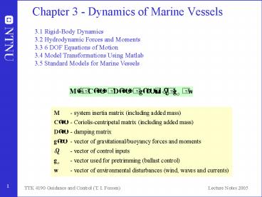
Chapter 3 - Dynamics of Marine Vessels
3.1 Rigid-Body Dynamics 3.2 Hydrodynamic Forces
and Moments 3.3 6 DOF Equations of Motion 3.4
Model Transformations Using Matlab 3.5 Standard
Models for Marine Vessels
2
3.1 Rigid-Body Dynamics
Coordinate free vector A vector defined by
its magnitude and direction but without reference
to a coordinate frame. Coordinate vector A
vector decomposed in the inertial reference
frame is denoted as vi Newton-Euler
Formulation Newton's Second Law relates mass m,
acceleration and force according
to where the subscript c denotes the center of
gravity (CG). Euler's First and Second
Axioms Euler suggested to express Newton's Second
Law in terms of conservation of both linear
momentum and angular momentum
according to
and are forces/moments about CG
is the angular velocity of frame b relative frame
i Ic is the inertia dyadic about the body's CG
3
3.1 Rigid-Body Dynamics

• When deriving the equations of motion it will be
  assumed that
• the vessel is rigid
• the NED frame is inertial
• The first assumption eliminates the consideration
  of forces acting between individual elements of
  mass while the second eliminates forces due to
  the Earth's motion relative to a star-fixed
  inertial reference system.
• For guidance and navigation applications in space
  it is usual to use a star-fixed reference frame
  or a reference frame rotating with the Earth.
  Marine vessels are, on the other hand, usually
  related to the NED reference frame. This is a
  good assumption since forces on marine craft due
  to the Earth's rotation
• are quite small compared to the hydrodynamic
  forces.

4
3.1.1Translational Motion

• Mass of a rigid body
• CG is defined as
• The position of the volume element dV is
• is constant over the volume

Body-fixed reference frame is fixed in the point
O and rotating with respect to the inertial
frame. is the vector from O to CG
5
3.1.1Translational Motion

• For marine vessels it is desirable to derive the
  equations of motion for an arbitrary origin O in
  the b-frame to take advantage of the vessel's
  geometric properties. Since the hydrodynamic and
  kinematic forces and moments are given in the
  b-frame, Newton's laws will be formulated in the
  b-frame as well. The b-frame coordinate system is
  rotating with respect to the i-frame (inertial
  system).
• The velocities of CG and O must satisfy
• It is common to assume that the NED frame is an
  approximate inertial frame by neglecting the
  Earth rotation and the angular velocity
  due to slow variations in longitude and
  latitude

6
3.1.1Translational Motion

• Decomposing
• into the b-frame under the assumption that
  , yields
• Hence, n-frame coordinates are obtained by using
  the rotation matrix
• Time differentiation, yields the acceleration of
  the CG in NED coordinates

7
3.1.1Translational Motion

• Euler's first axiom
• decomposed in the i-frame becomes
• 
  
• 
  assumes that NED is
  the inertial frame
• The acceleration decomposed in the n-frame was
  shown to be
• This gives Newtons law formulated with respect
  to the point O
• If the origin O of is chosen to coincide with the
  CG, we have
• rgb 0,0,0T fob fcb and vob
  vcb.

coordinate free representation
8
3.1.2 Rotational Motion (Attitude Dynamics)

• The derivation starts with the Eulers second
  axiom
• and the main result when decomposed in the
  i-frame under the previous assumptions is
• where Io is the inertia matrix
• where Ix, Iy, and Iz are the moments of inertia
  about the b-frame xyz-axes, and IxyIyx, IxzIzx
  and IyzIzy are the products of inertia defined
  as

9
3.1.2 Rotational Motion (Attitude Dynamics)

• Euler's equations if
• the attitude dynamics becomes
• Parallel Axes Theorem
• The inertia matrix about
  an arbitrary origin O is given by
• where is the inertia
  matrix about the body's CG.
• Proof see Fossen (2002).

10
3.1.3 Rigid-Body Equations of Motion
Component form (SNAME 1950)
11
3.1.3 Rigid-Body Equations of Motion
Matrix-Vector Form (Fossen 1991) Property
(Rigid-Body System Inertia Matrix)
generalized velocity
is the identity matrix is the
inertia matrix about O is the matrix cross
product operator
12
3.1.3 Rigid-Body Equations of Motion
Theorem (Coriolis-Centripetal Matrix from System
Inertia Matrix) Let M be a 66 system inertia
matrix defined as where M21M12T. Then the
Coriolis-centripetal matrix can always be
parameterized such that
by choosing where Proof see Sagatun and
Fossen (1991) or Fossen (2002).
13
3.1.3 Rigid-Body Equations of Motion

• Property (Rigid-Body Coriolis and Centripetal
  Matrix)
• The rigid-body Coriolis and centripetal matrix
  can always be represented such that
  is skew-symmetric, that is
• Application of the Theorem with MMRB yields the
  following expression for
• for which it is noticed that .

14
3.1.3 Rigid-Body Equations of Motion

• Three other useful skew-symmetric representations
  were derived by Fossen and Fjellstad (1995)
• Proof see Fossen and Fjellstad (1995).
• Notice that the there are no unique
  parametrization for the product
• such that becomes skew-symmetrix.

15
3.1.3 Rigid-Body Equations of Motion
Simplified 6 DOF Rigid-Body Equations of Motion

• Origin O coincides with the CG
• This implies that
  such that
• A further simplification is obtained when the
  body axes (xb,yb,zb) coincide with the principal
  axes of inertia. This implies that

16
3.1.3 Rigid-Body Equations of Motion
Simplified 6 DOF Rigid-Body Equations of Motion

• Rotation of the body axes such that Io becomes
  diagonal The body-fixed frame (xb,yb,zb) can be
  rotated about its axes to obtain a diagonal
  inertia matrix.
• Principal axis transformation The eigenvalues
  of Io are found from
• The modal matrix Hh1,h2,h3 is obtained from
  the right eigenvectors hi
• the coordinate system (xb,yb,zb) is then rotated
  about its axes to form a new coordinate system (x
  b,yb,zb) with unit vectors
• The new inertia matrix Io will be diagonal, that
  is

17
3.1.3 Rigid-Body Equations of Motion
Simplified 6 DOF Rigid-Body Equations of Motion

• The disadvantage with Approach (2) is that the
  new coordinate system will differ from the
  longitudinal, lateral, and normal symmetry axes
  of the vessel.
• The resulting model is
• It is, however, possible to let the body axes
  coincide with the principal axes of inertia, that
  is the longitudinal, lateral, and normal symmetry
  axes of the vessel, and still obtain a diagonal
  inertia matrix Io.
• Approach (3)

18
3.1.3 Rigid-Body Equations of Motion
Simplified 6 DOF Rigid-Body Equations of Motion

• (3) Translation of the origin O such that Io
  becomes diagonalThe origin of the body-fixed
  coordinate system can be chosen such that the
  inertia matrix of the body-fixed coordinate
  system will be diagonal. Let
• From the parallel axes theorem
• the diagonal must satisfy
• where xg, yg and zg must be chosen such that
• the remaing cross terms satisfy

19
3.2 Hydrodynamic Forces and Moments

• Radiation-Induced Forces (Zero-Frequency
  Approach)
• Forces on the body when the body is forced to
  oscillate with the wave excitation frequency and
  there are no incident waves (Faltinsen 1990)
• Added mass due to the inertia of the surrounding
  fluid
• Radiation-induced (linear) potential damping due
  to the energy carried away by generated surface
  waves
• Restoring forces due to Archimedes (weight and
  buoyancy)
• Faltinsen, O. (1991). Sea Loads on Ships and
  Offshore Structures, Cambridge.

20
3.2 Hydrodynamic Forces and Moments

• In addition to potential damping we have to
  include other damping effects like skin friction,
  wave drift damping, and damping due to vortex
  shedding
• Total hydrodynamic damping matrix
• The hydrodynamic forces and moments can be
  now be written as the sum of

21
3.2 Hydrodynamic Forces and Moments

• Environmental Disturbances
• In addition to the hydrodynamic forces and
  moments, the vessel will be exposed to
  environmental forces like
• wind
• Waves (Froude-Krylov/diffraction and wave drift)
• currents
• The resulting environmental force and moment
  vector is denoted as w.
• Resulting Model (Zero-Frequency/Low-Frequency
  Model)

22
3.2.1 Added Mass and Inertia

• Alternative approach to the Newton-Euler
  formulation Lagrangian mechanics
• Euler-Lagranges Equation (only for generalized
  coordinates)
• Kirchhoff's Equations in Vector Form (uses only
  kinetic energy / velocity)

generalized coordinates 6 DOF
difference between kinetic and potential energy
quaternions are not generalized coordinates
body velocities are not generalized coordinates
kinetic energy
23
3.2.1 Added Mass and Inertia

• Fluid Kinetic Energy (Zero-Frequency)
• The concept of fluid kinetic energy can be used
  to derive the added mass terms.
• Any motion of the vessel will induce a motion in
  the otherwise stationary fluid. In order to allow
  the vessel to pass through the fluid, it must
  move aside and then close behind the vessel.
• Consequently, the fluid motion possesses kinetic
  energy that it would lack otherwise (Lamb 1932).

24
3.2.1 Added Mass and Inertia
Property (Hydrodynamic System Inertia Matrix) For
a rigid-body at rest (U0), and under the
assumption of an ideal fluid, no incident waves,
no sea currents, and zero frequency, the
hydrodynamic system inertia matrix is positive
definite
Kirchhoff's Equations
25
3.2.1 Added Mass and Inertia
Hydrodynamic added mass forces and moments in 6
DOF The expressions are complicated and not to
suited for control design Hydrodynamic software
programs like WAMIT, VERES, and SEAWAY can be
used to compute the added mass terms The model
can be more compactly written using the added
mass system inertia matrix and the added
mass Coriolis and centripetal matrix
(Fossen 1991)
26
3.2.1 Added Mass and Inertia

• The added mass Coriolis and centripetal matrix is
  found by collecting all terms that are not
  functions of body accelerations (Sagatun and
  Fossen 1991)
• Property (Hydrodynamic Coriolis and centripetal
  matrix) For a rigid-body moving through an ideal
  fluid the hydrodynamic Coriolis and centripetal
  matrix can always be parameterized such that it
  is skew-symmetric
• by defining
• Example (Fossen 1991)

27
3.2.2 Hydrodynamic Damping

• Hydrodynamic damping for marine vessels is mainly
  caused by
• Potential Damping Radiation-induced damping .The
  contribution from the potential damping terms
  compared to other dissipative terms like viscous
  damping are usually negligible.
• Viscous damping Linear skin friction due to
  laminar boundary layer theory and pressure
  variations are important when considering the
  low-frequency motion of the vessel. Hence, this
  effect should be considered when designing the
  control system. In addition to linear skin
  friction, there will be a high-frequency
  contribution due to a turbulent boundary layer
  (quadratic or nonlinear skin friction). Ref.
  Faltinsen and Sortland (1987)
• Wave Drift Damping Wave drift damping can be
  interpreted as added resistance for surface
  vessels advancing in waves. This type of damping
  is derived from 2nd-order wave theory.

28
3.2.2 Hydrodynamic Damping

• Damping Due to Vortex Shedding D'Alambert's
  paradox states that no hydrodynamic forces act
  on a solid moving completely submerged with
  constant velocity in a non-viscous fluid. In a
  viscous fluid, frictional forces are present such
  that the system is not conservative with respect
  to energy. The viscous damping force due to
  vortex shedding can be modeled as

where U is the speed, A is the projected
cross-sectional area under water, Cd is the
drag-coefficient based, and is the water
density.
Kinematic viscosity coefficient
Reynolds number
29
3.2.2 Hydrodynamic Damping

• For low-speed applications like DP, quadratic
  damping can be modeled using the ITTC drag
  formalism in surge, and cross-flow drag in sway
  and yaw

Relative velocities
Ref. Faltinsen (1990)
2D drag coefficients Cd(x)
3D correction factors
30
3.2.2 Hydrodynamic Damping

• 6 DOF representation of MIMO quadratic drag

Total hydrodynamic damping
31
3.2.2 Hydrodynamic Damping

• Property (Hydrodynamic Damping Matrix) For a
  rigid-body moving through an ideal fluid the
  hydrodynamic damping matrix will be real,
  non-symmetric and strictly positive

Example For ships with xz-symmetry the surge
mode can be decoupled from the steering modes
(sway and yaw). Hence, the linearized damping
forces and moments (neglecting heave, roll, and
pitch) can be written (zero-frequency) For
low speed applications it can also be assumed
that NvYr such that DDT.
32
3.2.2 Hydrodynamic Damping
Dynamic positioning (station-keeping and
low-speed maneuvering) Linear damping
dominates Maneuvering (high-speed)Nonlinear
damping dominates

• The figure illustrates the significance of linear
  and quadratic
• damping for low-speed and high-speed applications.

33
3.2.2 Hydrodynamic Damping

• Example Nonlinear Damping Model for Maneuvering
  at Moderate SpeedIn Blanke (1981) a more
  detailed model including nonlinear coupling terms
  is proposed. This is a simplification of
  Norrbin's nonlinear model (Norrbin 1970).
  Motivated by this a more general expression
  (assuming that surge is decoupled) is
• Example Damping Model for Low-Speed Underwater
  VehiclesIn general, the damping of an underwater
  vehicle moving in 6 DOF at high speed will be
  highly nonlinear and coupled. Nevertheless, one
  rough approximation could be to assume that the
  vehicle is performing a non-coupled motion. This
  suggests a diagonal structure of D with only
  linear and quadratic damping terms on the
  diagonal
• As for ships quadratic damping can be neglected
  during station-keeping but not in high speed
  maneuvering situation

34
3.2.3 Restoring Forces and Moments

• In addition to the mass and damping forces,
  underwater vehicles and floating vessels will
  also be affected by gravity and buoyancy forces.
• In hydrodynamic terminology, the gravitational
  and buoyancy forces are called restoring forces,
  and they are equivalent to the spring forces in a
  mass-damper-spring system.
• In the derivation of the restoring forces and
  moments
• underwater vehicles (ROV, AUV, submarines)
• surface vessels (ships, semi-submersibles, and
  high-speed craft)
• will be treated separately.

35
3.2.3 Restoring Forces and Moments

• Underwater Vehicles
• According to the SNAME(1950) notation, the
  submerged weight of the body and buoyancy
  forceare defined as
• water density
• volume of fluid displaced by
  the vehicle
• m mass of the vessel including
  water in free floating space
• g acceleration of gravity

The weight and buoyancy force can be transformed
from NED to the body-fixed coordinate system by
36
3.2.3 Restoring Forces and Moments

• The sign of the restoring forces and moments
  and must be changed when
  moving these terms to the left-hand side of
• that is, the vector .
• Consequently, the restoring force and moment
  vector in the b-frame takes the form
• where

center of buoyancy center of gravity
37
3.2.3 Restoring Forces and Moments

• Main Result Underwater Vehicles
• 6 DOF gravity and buoyancy forces and moments

38
3.2.3 Restoring Forces and Moments

• Example Neutrally Buoyant Underwater Vehicles
  Let the distance between the center of gravity
  CG and the center of buoyancy CB be defined by
  the vector
• For neutrally buoyant vehicles WB, and this
  simplifies to
• An even simpler representation is obtained for
  vehicles where the CG and CB are located
  vertically on the z-axis, that is xbxg and
  ygyb. This yields

39
3.2.3 Restoring Forces and Moments

• Surface Vessels (Ships and Semi-Submersibles)
• For surface vessels, the restoring forces will
  depend on the vessel's metacentric height, the
  location of the CG and the CB as well as the
  shape and size of the water plane. Let Awp denote
  the water plane area and
• GMT transverse metacentric height (m)
• GML longitudinal metacentric height (m)
• The metacentric height GMi, where iT,L, is the
  distance between the metacenter Mi and center of
  gravity CG

Definition (Metacenter)The theoretical point at
which an imaginary vertical line through the CB
intersects another imaginary vertical line
through a new CB created when the body is
displaced, or tilted, in the water.
40
3.2.3 Restoring Forces and Moments

• For a floating vessel at rest, buoyancy and
  weight are in balance
• z displacement in heave
• z0 is the equilibrium position
• The hydrostatic force in heave will be the
  difference between the gravitational and
  buoyancy forces

where the change in displaced water is
is the water plane area of the
vessel as a function of the heave position
41
3.2.3 Restoring Forces and Moments

• For conventional rigs and ships, however, it can
  be assumed that
• is constant for small perturbations in z.
• Hence, the restoring force Z will be linear in z,
  that is

The restoring forces and moments decomposed in
the b-frame
z
Z
42
3.2.3 Restoring Forces and Moments

• The moment arms in roll and pitch can be related
  to the moment arms and in
  roll and pitch, and a z-direction force pair with
  magnitude

43
3.2.3 Restoring Forces and Moments

• Main Result Surface Vessels
• 6 DOF gravity and buoyancy forces and moments

44
3.2.3 Restoring Forces and Moments

• Linear (Small Angle) Theory for Boxed Shaped
  Vessels
• Assumes that are small such that

Linear dynamics
45
3.2.3 Restoring Forces and Moments

• The diagonal G matrix is based on the assumption
  of yz-symmetry. In the asymmetrical case G takes
  the form
• where

46
3.2.3 Restoring Forces and Moments
Metacenter M, center of gravity G and center of
buoyancy B for a submerged and a floating vessel.
K is the keel line.
47
3.2.3 Restoring Forces and Moments

• The metacenter height can be computed by using
  basic hydrostatics

M
For small roll and pitch angles the transverse
and longitudinal radius of curvature can be
approximated by where the moments of area
about the water planes are defined as
G
B
K
For conventional ships an upper bound on these
integrals can be found by considering a
rectangular water plane area AwpBL where B and L
are the beam and length of the hull
48
3.2.3 Restoring Forces and Moments

• Definition (Metacenter Stability)
• A floating vessel is said to be
• Transverse metacentrically stable if GMT
  GMT,min gt 0
• Longitudinal metacentrically stable if GML
  GML,min gt 0
• The longitudinal stability requirement is easy to
  satisfy for ships since
• the pitching motion is quite limited.
• The lateral requirement, however, is an important
  design criterion used to predescribe sufficient
  stability in roll to avoid that the vessel does
  not roll around. For instance, for large ferries
  carrying passengers and cars, the lateral
  stability requirement can be as high as GMT,min
  0.8 (m) to guarantee a proper stability margin in
  roll.
• A trade-off between stability and comfort should
  be made since a large stability margin will
  result in large restoring forces which can be
  quite uncomfortable for passengers.