
Electron%20probe%20microanalysis%20EPMA PowerPoint PPT Presentation
Title: Electron%20probe%20microanalysis%20EPMA
1
Electron probe microanalysisEPMA
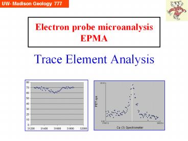
- Trace Element Analysis
2
Whats the point?
Whats the minimum detection limit for a
particular element or said otherwise, at what
point can be be sure that a small inflection
above the surrounding background really is a
peak? What kind of confidence level should be
place on such a number?
3
Definitions
Generally, WDS can achieve limits of detection
of 100 ppm in favorable cases, with 10 ppm in
ideal situations where there are no peak
interferences and negligible matrix absorption.
(Goldstein et al., p. 341)
Major gt10 wt Minor 1-10 wt Trace lt1 wt
No Zn ... but at what level of confidence?
4
Trace elements .... and trace elements
In the real world, the definition of
trace element analysis is sometimes broader
than the strict quantitative analysis of ppm
level elements in one microvolume (micron
interaction volume). Many individuals desire to
use EPMA to tell them about the distribution of
trace elements in their materials, e.g. where
the 30 ppm of Pb is in a cast iron. There are two
possibilities the 30 ppm is spread uniformly
throughout the material, or in fact most of the
material has probably lt1 ppm of Pb, but a small
fraction of the volume has phases that have Pb at
major element levels.The question is then, are
they at least the size of the interaction volume
and if so, where are they. Our discussion here
will deal with all these aspects.
5
A little background
- Interest in trace elements dove tails with the
develop of techniques that could achieve
better/quicker/cheaper/more precise/small volumes
of said elements. - From the 1960s on, geochemists and petrologists
developed increasing interest in trace element
partitioning between fluids/melts and minerals.
The electron microprobe became the instrument of
choice for characterizing the trace levels in
doped experiments . - There has been an interest in trace elements
in certain minerals to assist in the search for
ore bodies that contain said elements. A related
research field is locating the naturally-occurring
minerals that are responsible for certain levels
of groundwater contamination (e.g. As).
6
How low can we go?
The USNM olivine standard above (San Carlos, Mg.9
Fe.1SiO4) has a published Ca content of lt0.04 wt
( 400 ppm). This scan was acquired at 20 keV,
30 nA, with 10 seconds per channel. Clearly there
is a peak at the Ca Ka position (24 cps),
somewhat above the background (10 cps). At
what point can we say with 99 confidence that
there is a statistically significant peak?
7
MDL Equations - 1
- The key concept here is minimum detection limit
(MDL), i.e., what is the lowest concentration of
the element present that is statistically above
the background continuum level by 3 sigma
(commonly accepted level). - There are (at least) two equations used to define
the MDL - the first uses the Student t test values
- where the detection limit CMDL is in wt, CSstd
wt ,bar NSave. peak cts on std,bar NSBbkg cts
on std, SC std dev of measured values and
nnumber of data points - the second, which is probably more wider used,
was developed by Ziebold (1967) - where nnumber of measurements, Tseconds per
measurement, Ppure element count rate, P/B for
pure element, and amatrix correction (a -factor
or ZAF).
Goldstein et al., p. 500, equation 9.84
Goldstein et al., p. 500, equation 9.85
8
MDL Equations - 2
- There are several points to be made about these
two equations - the first (Student t test) equation only works
for the average of several measurements, since it
uses SC, the average of several measurement. This
calculation is useful in that special case. - however, as many times as not, a specific area
or region is only measured once (e.g., a linear
traverse across a zoned crystal), and the second
equation is the appropriate one to use. - note in the second equation, the term P times
P/B appears in the denominator. As P2/B
increases, the MDL decreases (the lower, the
better!). This P2/B term is called the figure of
merit for trace element work. - following some discussions with John Valley
about the traditional (second) equation and how
the peak and background used in it were from the
pure element standardnot the unknown, I went
back to first principles and derived the equation.
9
Deriving the MDL equation-1
1. We need to determine the precision of the
background value for the unknown, i.e. for a
given background value, how big is the
statistical error bar (counting statistic, 3
sigmas) above it. So here, is it large as on the
right below, or is it small as on the right?
10
Deriving the MDL equation-2
2. Let us consider Ca Ka peak on our
olivine. We measure the background and get 9
cts/sec. The 1 sigma value however is calculated
from TOTAL counts, NOT count rate. So we must
multiply 9 cts/sec by the time, 10 seconds, and
we get 90 counts. 1sSq.Rt. of 90 9.5 counts, so
3s 28.5. Well use 3 s for now, the 99.7
confidence level. Ergo, our MDL for Ca in the
olivine is 29 counts above background, over 10
seconds (or if plotted on the wavescan where data
are in cts/sec, it would be a value of 3 cps (the
left purple marker). Note we havent said one
word about count rate on a standard, and we have
figured out the minimum detection limit for Ca in
our unknown -- though we dont know what that mdl
of 3 cts/sec translates to in ppm or wt).
11
Deriving the MDL equation-3
3. However, we usually want to translate those
raw counts into a more usable number, i.e. so
many ppm. For that, we need some reference
intensity counts for Ca Ka. We then count Ca ka
peak and backgrounds for the same time (10 sec)
on CaSiO3 (38.6 wt Ca) and find a count rate of
6415 cts/sec on the peak and 16 cts/sec on the
background. 4. So what is 2.9 cts/sec equal to
in elemental wt? We create a pseudo k-ratio
where we take the statistical uncertainty of the
background counts (square root, i.e. 1 sigma)
divided by the Peak-Bkg of the standard counts on
the element peak of interest and multiply by 3
(for 3 sigma, 99 confidence) and the ZAF of each
and then by the composition C of the standard.The
mdl will be in whatever units C is in.
12
Deriving the MDL equation-4
This is virtually the same result as the
single line detection limit provided by Probe
for Windows (0.015 wt, shown on next slide),
derived from the Ziebold equation. It would
appear that the Ziebold equation is not exactly
correct, for we must really be concerned with the
background precision of the unknown, and the
background level of the standard could be several
times higher or lower. Going back and re-reading
Ziebold, we find two interesting statements that
the equation gives a measure of the
detectability limit and there is more than one
way to define a detectability limit. Both are
correct, and yes, the equation gives an
approximation of the detection limit -- but not
the limit per se.
13
MDL in olivine - single line
Good totals
Excellent stoichometry
These are the single line detection limits,
calculated with Ziebolds equation (Goldstein, eq
9.85, p. 500)
14
MDL in olivine - average
For a homogeneous sample, it is legal to add
together all the counts, which gives greater
precision and a lower detection limit, e.g. 110
ppm here for Ca at 99 ci.
This is a handy chart that shows what kind of
counting time would be required, under the same
analytical conditions, to achieve a lower
detection limit. For example, to get a mdl of 25
ppm, youd need to count for 5 minutes on the Ca
peak and then background (for each of 10 spots).
The current analysis here was a little over 1
minute per spot (thus, about 12 minutes for a mdl
of 110 ppm. For 25 ppm, it would add an
additional 100 minutes to the analysis time.
15
Figure of Merit
Probers in Australia have much interest in
pushing the lower limits of EPMA detection, for
mineral exploration research.Utilizing extreme
operating conditions (50 kV, 475 nA, 10 minute
counts) they have achieved mdls below 5 ppm for
some elements.
They utilize a figure of merit of P2/B as a
measure of how to achieve lower mdl (the higher
the P2/B ).
From our first principles derivation, we can see
that the P comes from the standard, the B from
the unknown.
From Advances in Electron Microprobe
Trace-Element Analysis by B.W. Robinson and J.
Graham, 1992, ACEM-12
16
Keys to low detection levels
- Maximize counts by utilizing
- Highest currents feasible (concern beam damage)
- Highest E0 as feasible (concern increased
penetration/range) - Longer count times
- Correctly determine background locations
- Correct for unavoidable on-peak interferences
within the matrix correction
Donovan, Snyder and Rivers, 1993, An improved
interference correction for trace element
analysis, Microbeam Analysis, 2, 23-28.
17
Backgrounds traces can overlap traces
Correct locating of background positions is
particularly important in trace element work, as
both first order and higher order peaks can cause
incorrect assessment of background level. Here,
scans of the 3 Caltech/MAS trace element glass
standards are overlain. (Xe L edge present as a
Xe gas sealed counter used.)
From Carpenter, Counce, Kluk, and Nabelek,
Characterization of Corning Standard Glasses
95IRV, 95IRW and 95IRX NIST/MAS Workshop, April
2002.
18
Backgrounds Pb Ma in Monazite
Here the Th Mz1 and 2nd order La La1 peaks fall
close to potential backgrounds for Pb Ma.
Monazite (Ce,La,REE,Th)PO4 has been used for age
dating, using U, Th and Pb concentrations.
19
Backgrounds ... holes
Probers in Australia, interested in detecting
trace levels of gold in certain minerals,
discovered a hole in the background about 200
sin theta units below the Au La position. (This
scan was on SrTiO3, on the LIF crystal).
20
Trace elements as fingerprints apatite in
bentonites
Crystals were separated from clay mixed
population (zircons, white apatites, yellow in
false color mosaic BSE image) mounts in 4 mm plug
(above).
(Research of Norlene Emerson.)
A range of trace elements were analyzed in
bentonites (very old volcanic ash), in order to
verify common stratigraphic horizons in
Ordovician sediments. 40-60 ppm mdls were
achieved with 20 second counts and 60 nA currents.
21
Where is the ...Arsenic?
Some groundwaters in northeast Wisconsin have
elevated Arsenic (8 mg/L), and EPMA is being used
to help understand the source. Aquifer strata
contain mineralized zones (500-80 ppm whole
rock), mainly marcasite (FeS2) and quartz. X-ray
maps (PfW-MAN) were acquired overnight for Fe, S,
Si, O and As. They showed that As is located on
the edge of some quartz grains. Here, a
rectangular area was mapped at 10 mm intervals.
(Research of Toni Simo,Katie Thornberg, Selena
Mederos)
22
Pb in Cast Iron
Pb Ma
C Ka
This cast iron has 100 ppm of Pb in the bulk
analysis, and the question was which phase did it
reside in. The working hypothesis was that it was
associated with graphite dendrites. A full
quantitative X-ray map (backgrounds acquired) was
acquired overnight (conditions 15 keV, 300 nA,
150 seconds each on Pb peak and bkg). The mdl
for Pb is 200 ppm (.02 wt).
Fe Ka
(Research of Jun Park, Carl Loper and John
Fournelle.)
23
X-ray mapping of irregularly positioned/shaped
zircon grains
- Mounted in epoxy need to avoid melting epoxy
with high currents! - Define polygon boundary
- Select point spacing interval
- Fully automated quantitative EPMA
- Software contouring or 3D surface mapping
(Surfer)
24
Huckleberry Ridge Tuff Zircon grain A(2 Ma,
2500 km3, normal d18O)
BSE
CL
BSE
- Th and U Ma (PET)
- 18 keV, 400 nA
- 94 points
- 10 elements
- 11 mm spacing
- 50 sec on peak 50 sec on bkgs 8 hours
total time - mdl 130 ppm (.013 wt)
U wt
Th wt
(Research of Ilya Bindeman, John Valley and John
Fournelle)
25
Standards validating trace element procedure
- There is an issue of trace element accuracy on
unknowns, where the standard for the element of
interest was at a high level. Such a standard
should be used for peaking the spectrometer and
acquiring standard counts, but it is recommended
that a secondary trace level standard be also
analyzed to validate the procedure. - Such secondary standards could be
- Synthetic glasses such as the Caltech/MAS
95IRV,W and X glasses NIST glasses and metals
Ni-Cr diopside glass, etc. - Minerals and glasses analyzed by ion probe
26
Comparison Trace elements by WDS vs EDS
WDS is clearly the better method for acquiring
trace element data, by an order of magnitude or
so compared to EDS.
Goldstein et al, 1992, p. 501
Recommended
