
Operational fully automated preliminary classification of multispectral satellite imagery PowerPoint PPT Presentation
1 / 113
Title: Operational fully automated preliminary classification of multispectral satellite imagery
1
Operational fully automated preliminary
classification of multi-spectral satellite imagery
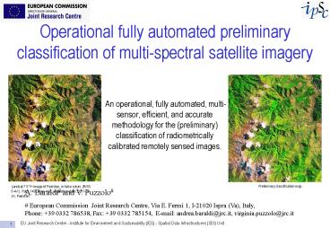
- An operational, fully automated, multi-sensor,
efficient, and accurate methodology for the
(preliminary) classification of radiometrically
calibrated remotely sensed images.
Landsat 7 ET image of Pakistan, in false colors
(RGB 5-4-1). Path 149, Row 036, acquisition
date 2001-09-30, Pakistan
Preliminary classification map.
A. Baraldi and V. Puzzolo European
Commission Joint Research Centre, Via E. Fermi
1, I-21020 Ispra (Va), Italy, Phone 39 0332
786538, Fax 39 0332 785154, E-mail
andrea.baraldi_at_jrc.it, virginia.puzzolo_at_jrc.it
2
Presentation overview
- Preliminary image classification concepts and
definitions. - Fully automated preliminary classification
operational system properties. - Implementation details.
- Application domain of the proposed classifier.
- Application examples.
- Quantitative map comparison with reference
samples extracted from CORINE2000 and Google
Earth. - Conclusions and future developments.
3
Preliminary spectral image classification
- Prior knowledge-based image classification ?
Prior to any image data analysis and without
exploiting any ground truth (reference) sample. - In practice, at purchase time, the user receives
Preliminary spectral map (semantic labeled image
pixels/ objects/ strata) vs traditional image
simplification via asemantic segmentation.
Acquired raw image
Landsat 7 ETM scene. False color image (R band
TM5, G band TM4, B band TM1).
Output map, in pseudo colors, generated from the
calibrated image.
Noteworthy, the proposed prior spectral
knowledge-based classifier is by no means
alternative to traditional data clustering, image
segmentation, and supervised classification
algorithms, to be rather employed in cascade to
spectral rule-based mapping on a stratified,
application-dependent basis.
4
Preliminary image classification concepts and
definitions
- Primal sketch (Preliminary map) of an input image
in the Marr sense (4, 1980) ? Image
simplification stage. - A primal sketch explicitly reveals kernel
(i.e., reliable) information about geometrical
distribution and organization of either color or
brightness changes. - Proposed solution Prior (to data observation)
spectral knowledge-based (i.e., spectral
rule-based) modular classifier capable of
modeling - known reflective properties of surface types in
the electromagnetic spectrum, and - within-class variability in spectral response
(e.g., due to atmospheric effects, if
top-of-atmosphere reflectance rather than surface
reflectance properties are investigated).
5
Preliminary image classification concepts and
definitions
- Implicit requirement of the proposed prior
spectral knowledge-based classification solution - Prior (to data observation) spectral
knowledge-based modular classifiers (as well as
non-supervised decision trees) may be defined
solely on analysit expertise if and only if they
rely upon datasets that are both - Well understood and
- Well behaved, namely, radiometrically calibrated
into top-of-atmosphere (TOA) reflectance (not
radiance!). It is well-known that the absolute
radiometric calibration of DNs into physical
quantities, like the TOA reflectance - Increases the consistency of RS imagery
(inter-image comparability) through time and
different satellite sensors by accounting for
seasonal and latitudinal differences in solar
illumination - Provides (reasonably) linear relationships
between the leaf area index (LAI) and a great
variety of well-known vegetation indices (VIs)
whereas those between LAI and the same vegetation
indices calculated from TOA reflectance are
nonlinear 6.
6
Preliminary image classification concepts and
definitions
- Examples of a reference dictionary of spectral
signatures that is both i) well understood, and
ii) well behaved, namely, radiometrically
calibrated into top-of-atmosphere (TOA)
reflectance (not radiance!), rescaled into range
0, 255.
Expose bare rock
Thick cloud (cumulus)
6
7
Preliminary image classification concepts and
definitions
- Second stage in remotely sensed image
understanding. - Hierarchical land cover classification system
exploiting i) raw image data, ii) kernel image
information (e.g., the preliminary spectral map),
and iii) image features from additional
information domains, e.g., - Texture visual effect generated from the
spatial variation of gray values in a 2-D image
domain. - Geometric attributes of (connected) objects,
e.g., area, shape, compactness, straightness of
boundaries, elongatedness, number of vertices
(estimated from skeletonization), etc. - Morphological attributes of (connected) objects,
namely, known shaped and sized bright (respect.,
dark) objects in a darker (respect., brighter)
background or vice versa. - Color/Brightness attributes of objects (e.g.,
mean, standard deviation, etc.). - Spatial non-topological relationships between
objects (e.g., distance, angle/orientation,
etc.). - Spatial topological relationships between
objects (e.g., adjacency, inclusion, etc.).
8
Product mosaic generation based on the
preliminary image classification complete
processing chain
- Mosaics of scientific quality to be input with
- MS rad. calib. imagery
- Value added products (e.g., Greenness)
- Classification maps
Orthorectification geometric correction
Image mosaics of scientific quality at global
scale
Multi-spectral raw image geometrically corrected
Mosaic of enhanced pictorial quality (by means of
a stratified histogram matching technique)
Visually enhanced image mosaic at global scale
(Automatic fuzzy rule-based, semi-automatic,
self-supervised) 2-stage classification
Preliminary classification stage (fully
automated)
Multi-spectral TOA reflectance image
Spectral preliminary map
8
9
Operational system properties
- It belongs to the public domain A. Baraldi, V.
Puzzolo, P. Blonda, L. Bruzzone, and C.
Tarantino, "Automatic spectral rule-based
preliminary mapping of calibrated Landsat TM and
ETM images," IEEE Trans. Geosci. Remote
Sensing, vol. 44, no. 9, pp. 2563-2586, Sept.
2006. - Operational spectral rule-based classifier (SRC)
IDL (JRC), c implementations (MEEO s.n.c.). - Suitable for mapping either
- 1st version, LSRC Landsat 5 TM and 7 ETM-like
imagery (e.g., ASTER, MODIS, CBERS, aerial
hyperspectral optical sensors Specim AISA DUAL,
Itres SASI 600 and CASI 1500, Galileo Avionica
SIM-GA) or - 2nd version, SSRC SPOT-4/5-like imagery (e.g.,
IRS-1C, IRS-1D, IRS-P6), or - 3rd version, AVSRC AVHRR-like imagery (e.g.,
Meteosat 2 Generation, MSG, ENVISAT AATSR), or - 4th version, ISRC IKONOS-like (e.g.,
QuickBird-1, OrbView-3, TopSat, RapidEye (to be
launched), FORMOSAT-2, KOMPSAT-2, ALOS AVNIR-2,
PLEIADES (to be launched)). - where
- RS images are radiometrically calibrated
into planetary (top-of-atmosphere,
exoatmospheric) reflectance and at-satellite
temperature (if any).
10
Operational system properties
- SRC adopts the following classification scheme.
- A discrete and finite set of six target land
cover classes, namely - Water/shadow.
- Snow/ice.
- Clouds.
- Vegetation.
- Bare soil/built-up.
- Outliers.
- A set of rules, or definitions, or properties for
assigning class labels. - Pixel-based (context-insensitive), which is
tantamount to saying purely spectral, either
chromatic or achromatic. - Prior knowledge-based (non-adaptive).
- This classification scheme is
- Mutually exclusive, i.e., each mapped area falls
into one and only one category. - Totally exhaustive (which implies that outliers
must be explicitly dealt with by class others).
In other words, SRC provides a complete partition
of an input RS image.
11
Operational system properties
- Fully automated, i.e, it requires a) no free
parameter and b) no reference (supervised) data
set of examples (i.e., no ground truth data) ?
Push-and-go (press-and-run) button-like
implementation. - Spectral prior knowledge-based, exclusively.
- No inductive data learning mechanism, neither
unsupervised (e.g., data clustering) nor
supervised (e.g., data classification). - Non-iterative (1-pass classification).
- It is based on prior spectral knowledge driven
from a dictionary of real-world spectral
signatures in planetary reflectance which account
for atmospheric effects. - It is implemented as a set of fuzzy rules capable
of modeling the prior spectral knowledge. - It is pixel-based. It detects small but genuine
image details, although it is not affected by the
traditional salt-and-pepper classification noise
effect.
12
Operational system properties
- It is computationally efficient, requiring
approximately 2 min per Landsat scene (from data
calibration to output map generation, c
implementation) ? Suitable for real-time
(on-line) image classification applications. - World wide web on-line customer service
satisfaction on demand. - Low- and high-level image processing capabilities
developed on-board future intelligent earth
observation satellites. - It is accurate (e.g., Overall classification
accuracy, OA 98.2 0.0 in a vegetation/non-vege
tation binary classification task at regional
scale in central Italy). - Up-scalable to (near-)hyperspectral sensors like
ASTER, MODIS, MSG, etc. (cascade implementation).
12
13
Operational system properties
- Up to now, the four implemented system versions
(three, downscaled) are capable of generating - Landsat-like, LSRC. Three standard preliminary
classification maps featuring different degrees
of informational granularity 85, 41, or 16
spectral categories (vegetations, rangelands,
bare soils, water/shadow, clouds, snow,
greenhouses, pitbogs, etc.) - SPOT-like, SSRC. Three standard degrees of
informational granularity 59, 35, or 14 spectral
categories. - AVHRR-like, AVSRC. Three standard degrees of
informational granularity 73, 37, or 15 spectral
categories. - IKONOS-like, ISRC. Three standard degrees of
informational granularity 46, 25, or 11 spectral
categories. - Value-added products consisting of continuous
spectral indexes potentially useful for further
application-dependent image analysis. - Greenness (? Leaf Area Index) (New formulation! 1
VIS, 1 NIR, and 1 MIR channels are required!!!
Minimum spectral resolution SPOT-like!!!), not
computed by IKONOS-like. - Canopy chlorophyll content.
- Canopy water content, not computed by
IKONOS-like. - Water/shadow/snow (!) index, not computed by
IKONOS-like. - Vegetation/Non-vegetation binary mask.
- Bare soil binary mask.
- Urban area candidate pixels.
14
Operational system properties Greenness ? Leaf
Area Index (LAI)
The second derivative of canopies centered on the
red and NIR wavebands are highly related to Leaf
Area Index (LAI) regardless of the different
backgrounds (burned and unburned). (Li et al.,
1993). It is computed using three wavebands
centered around the max first derivative of a
vegetation reflectance red edge (Red Edge
Inflection Point, REIP).
Bare Soil Index ETM5 / ETM4
Vegetation Index ETM4 / ETM3
15
Classification systems properties Output
product overview
High
Output map product types 1 to 3 Standard
preliminary classification maps featuring
different degrees of informational granularity
72, 38, or 15 spectral categories in the Landsat
system version (49, 32, or 13 in the SPOT system
version and 70, 37, 15 in the AVHRR system
version, respectively). Label indexes are
monotonically decreasing with category-specific
biomass estimates (label 1 SVVHNIR, label 2
SVHNIR, etc.).
Biomass
72 SCs
Input image
Output value-added product types 4 to
7 Value-added products suitable for stratified
second-stage supervised classification, image
segmentation, data clustering.
a) (Novel) Greenness
b) Canopy Water Content
c) Canopy Chlorophyll Content (NDVI)
d) Water/Shadow spectral index
Low
16
Classification systems properties Output
product overview
Landsat 7 ETM image of Trentino (Path 193, Row
028, acquisition date 1999-09-13) depicted in
false colors (RGB5-4-1).
Classification map, 72 SCs maximum sensitivity
in LCC detection.
Classification map, 38 SCs.
Classification map, 15 SCs maximum reduction of
fragmentation (scene noise) in the
classification map.
Observation The best informational granularity
(fragmentation) is user- and application-dependent
.
17
Classification system scalability to other sensors
Scalability of the Landsat rule-based classifier
to SPOT-4 and -5 (done! From 85 to 59 output
categories), ASTER (done! 85 categories) and
MODIS (done! 85 categories).
18
Classification system scalability to other sensors
Scalability of the Landsat rule-based classifier
to NOAA AVHRR (done! From 85 to 73 output
categories) and MSG (done!).
19
Classification system scalability to other sensors
Based on theoretical considerations, little
effective in discriminating between veg. and
non-veg. land covers based on spectral
properties, exclusively!
- Problem
- Landsat ? SPOT adaptation causes a loss in
spectral resolution (potentially compensated by
an increase in spatial resolution). In
particular - In VIS, one band (Blue) is lost, out of tree ?
loss in the discrimination capability of water
types. - In MIR, one band is lost out of two ? loss in the
discrimination capability of non-veg. spectral
categories. - In TIR, one band is lost out of one ? difficult
discrimination of snow and clouds from
non-veg.spectral categories (e..g, bright barren
soils).
20
Baseline (preliminary) thematic mapping
Symbolic meaning of spectral categories
- Baseline spectral map ? Preliminary (spectral)
map ? Primal sketch (in the Marr sense 4).
Symbolic (semantic) meaning of informational
primitives
BEST CASE
WORST CASE
Users degree of supervision
21
Symbolic (semantic) meaning of spectral
categories Some examples
22
Relations between spectral categories and
vegetation land covers
23
Rule-based system implementation
24
Input space partitioning (irregular but
complete) through fuzzy sets
1
Fuzzy membership ? 0, 1
Scalar input feature F1? ?, e.g., NDVI ? -1, 1
0
LOW
MEDIUM
HIGH
LOW
F2? ?, e.g., band TM4 ? 0, 255
HIGH
25
Rule-based system implementation
- Block diagram two-stage spectral rule-based
system architecture. - Feature extraction (e.g., NDVI, NDBSI, NDSI,
etc.) - Relational properties (, , etc.) among
class-specific reflectance values in different
portions of the electromagnetic spectrum. - Fuzzy set (High, Medium, and Low) computation.
- Combination of fuzzy sets and relational
properties. - Software written in IDL (ITT Visual Solutions).
PRE-PROCESSING LEVEL
PRE-PROCESSING LEVEL
PRE-PROCESSING LEVEL
1st LEVEL OF ANALYSIS
1st LEVEL OF ANALYSIS
1st LEVEL OF ANALYSIS
2nd LEVEL OF ANALYSIS
2nd LEVEL OF ANALYSIS
2nd LEVEL OF ANALYSIS
26
Radiometric calibration
The proposed classifier employs Landsat 5 TM and
Landsat 7 ETM images calibrated into planetary
(or top-of-atmosphere, TOA) reflectance and
at-satellite temperature values. The calibration
is carried out as follows.
ETM 1-5 and 7
ETM 62
Calculate band-specific gain
TOA Radiance (Li)
Calculate the cosine (cosun) of the solar zenith
angle ?z (90 sunel)
TOA Reflectance (si)
Temperature (T)
Convert Reflectance (si) from float 0,1 to
byte 0,255
Convert Temperature (T) from Kelvins to
Celsius degrees in byte 0,255
Radiances LMaxi, LMini, and DNs QcalMaxi 255,
QcalMini 1, to be read from metadata. sunel
sun elevation angle, provided in the metadata
(.met) file.
d? 1 Earth-sun distance (refer to Landsat 7
Handbook). Esuni Mean solar exoatmospheric
irradiance (refer to Landsat 7 Handbook).
PRE-PROCESSING LEVEL
PRE-PROCESSING LEVEL
PRE-PROCESSING LEVEL
1st LEVEL OF ANALYSIS
1st LEVEL OF ANALYSIS
1st LEVEL OF ANALYSIS
2nd LEVEL OF ANALYSIS
2nd LEVEL OF ANALYSIS
2nd LEVEL OF ANALYSIS
27
Application domain of the proposed classifier
- One-shot quick-look (baseline) thematic mapping
of wide surface areas (e.g., 65000 km2 per
Landsat scene) provided with little or no ground
truth. - To guide the user selection of reference samples
required for supervised inductive learning
classification. - To drive single-date second-stage stratified
image processing algorithms, where the
stratum-specific decision problem becomes easier
to solve. For example - Non-lambertian class-specific topographic effects
correction (illumination condition normalization)
? pre-processing chain with feed-back mechanism. - Image pair relative calibration.
- Segmentation.
- Clustering.
- Supervised classification.
28
Application domain of the proposed classifier
- To provide multitemporal image classification
tasks with an additional information source ?
semantic-based land cover change detection (based
on a post-classification change detection
approach). - To allow querying an imagery database for
geospatial semantic pixels, objects and strata,
e.g., to minimize purchased risks resulting from
undesired cloud cover or surface conditions. - Current state-of-the-art in content-based image
database retrieval (CBIR) - Visual query by pictorial data examples.
- Relevance feedback (selected images at every
round are flagged as either positive or negative
examples).
29
eCognition image segmentation and object-based
classification
- eCognition User Guide 4, 2004.
Chromatic or achromatic Input Image
Informational primitive pixel withouth any
semantic label
Hierarchical piecewise constant image
segmentation (includes no texture model)
Informational primitive segment withouth any
semantic label
. . .
. . .
. . .
Informational primitive segment with a semantic
label
30
Stratified image segmentation/ clustering/supervis
ed classification
- Hierarchical pixel- and object-based Davis
classification approach 11, 2003.
Informational primitive pixel withouth any
semantic label
Informational primitive pixel/ segment/ stratum
with a semantic label
Informational primitive segment with a semantic
label
?4
?5
?3
?2
?6
?1
Informational primitive pixel/ segment/ stratum
with a semantic label
?7
31
Stratified image segmentation/ clustering/supervis
ed classification
- Hierarchical pixel- and object-based Baraldi
classification approach, 2007.
Informational primitive pixel withouth any
semantic label
Informational primitive pixel/segment/stratum
with a semantic label
Informational primitive segment with a semantic
label
?4
?5
?3
?2
?6
Informational primitive pixel/segment/stratum
with a semantic label
?1
?7
32
Traditional and novel approach to image
classification
Traditional object-based image classification
approach (e.g., eCognitions)
Image segmentation
Segment-based fuzzy classification
(Connected) Segment without a semantic label
Pixel without a semantic label
Segment / Stratum with a semantic label
Marrs primal sketch (or preliminary map) of the
input image, which explicitly reveals information
about geometrical distribution and organization
of either color or intensity changes ? The
informational complexity of the image is reduced.
Novel pixel- and object-based image
classification approach (e.g., Davis)
Stratified Class-specific Fuzzy rule-based
classification
Preliminary pixel-based classification
Pixel/ Segment / Stratum with a final semantic
label
Pixel / Segment / Stratum with a preliminary
semantic label
Pixel without a semantic label
De-fuzzification
33
Application domains 1 and 2. Baseline map
generation / ROI extraction from Landsat 7 ETM
imagery. Example a Israel.
Fig. B. Output map generated from Fig. A by the
spectral rule-based classifier capable of
detecting 45 classes. Adopted pseudo colors are
the following. Green tones vegetation and
rangeland, Brown and grey color shades barren
land and built-up areas, Blue tones water types,
etc.
Fig. A. Landsat 7 ETM scene. False color image
(R band TM5, G band TM4, B band TM1). Path
174, Row 038, acquisition date 2002-03-08, West
bank area , Israel.
34
Zoomed area. Example a Landsat 7 ETM, Israel.
Fig. C. Zoomed area extracted from Fig. A. False
color image (R band TM5, G band TM4, B band
TM1). Path 174, Row 038, acquisition date
2002-03-08, West bank area , Israel.
Fig. D. Zoomed area extracted from the 45-class
output map shown in Fig. B. Adopted pseudo colors
are the following. Green tones vegetation and
rangeland, Brown and grey color shades barren
land and built-up areas, Blue tones water types,
etc.
35
Application domains 1 and 2. Baseline map
generation / ROI extraction from Landsat 7 ETM
imagery. Example b Pakistan.
Fig. B. Output map generated from Fig. A,
consisting of 45 spectral categories. Adopted
pseudo colors are the following. Green tones
vegetation and rangeland, Brown and grey color
shades barren land and built-up areas, Blue
tones water types, White tones clouds, Light
blue tones snow and ice, etc.
Fig. A. Landsat 7 ETM scene. False color image
(R band TM5, G band TM4, B band TM1). Path
149, Row 036, acquisition date 2001-09-30,
Pakistan.
36
Zoomed area. Example b Landsat 7 ETM, Pakistan.
Fig. C. Zoomed area extracted from Fig. A. False
color image (R band TM5, G band TM4, B band
TM1). Path 149, Row 036, acquisition date
2001-09-30, Pakistan.
Fig. D. Zoomed area extracted from the 45-class
output map shown in Fig. B. Adopted pseudo colors
are the following. Green tones vegetation and
rangeland, Brown and grey color shades barren
land and built-up areas, Blue tones water types,
White tones clouds, Light blue tones snow and
ice, etc.
37
Application domains 1 and 2. Baseline map
generation / ROI extraction from Landsat 7 ETM
imagery. Example c Denmark.
Fig. B. Output map generated from Fig. A,
consisting of 45 spectral categories. Adopted
pseudo colors are the following. Green tones
vegetation and rangeland, Brown and grey color
shades barren land and built-up areas, Blue
tones water types, etc.
Fig. A. Landsat 7 ETM scene. False color image
(R band TM5, G band TM4, B band TM1). Path
197, Row 021, acquisition date 2001-05-09,
Denmark.
38
Zoomed area. Example c Landsat 7 ETM, Denmark.
Fig. D. Zoomed area extracted from the 45-class
output map shown in Fig. B. Adopted pseudo colors
are the following. Green tones vegetation and
rangeland, Brown and grey color shades barren
land and built-up areas, Blue tones water types,
etc.
Fig. C. Zoomed area extracted from Fig. A. False
color image (R band TM5, G band TM4, B band
TM1). Path 197, Row 021, acquisition date
2001-05-09, Denmark.
39
Application domains 1 and 2. Baseline map
generation / ROI extraction from Landsat 7 ETM
imagery. Example d image mosaic of Italy.
Output map generated by the JRC-IES from a mosaic
of Landsat 7 ETM images of Italy, 45 spectral
categories.Adopted pseudo colors are the
following. Green tones vegetation and rangeland,
Brown and grey color shades barren land and
built-up areas, Blue tones water types, etc. On
the left and right side, a comparison between a
Landsat true colour image on top versus a
classified Landsat image area in pseudo colors on
bottom.
40
Application domains 1 and 2. Baseline map
generation / ROI extraction from SPOT-5 imagery.
Example e Trentino (Italy).
Fig. B. Output map generated from Fig. A,
consisting of 49 spectral categories. Adopted
pseudo colors are the following. Green tones
vegetation and rangeland, Brown and grey color
shades barren land and built-up areas, Blue
tones water types, etc.
Fig. A. SPOT-5 scene. False color image (R band
4, G band 3, B band 1). Acquisition date
2006-31-08, Trentino (Italy), spatial resolution
10 m.
41
Application domains 1 and 2. Baseline map
generation / ROI extraction from SPOT-5 imagery.
Example f and g Kenya and Kashmir.
SPOT-5 image of Kenya (acquisition date
2004-09-20), spatial resolution 10 m. On the
right, a zoomed image of Nairobi.
SPOT-5 image of Kashmir (acquisition date
2005-10-21), spatial resolution 10 m. On the
right, a zoomed image portion.
Preliminary spectral map in pseudo colors. On the
right, a zoomed map portion.
Preliminary spectral map in pseudo colors. On the
right, a zoomed map portion.
42
Application domains 1 and 2. Baseline map
generation / ROI extraction from SPOT-5 imagery.
Example g Kashmir.
- GMOSS Kahmire testcase Processing chain
- SPOT image radiometric calibration.
- Automated classification map generation from the
calibrated SPOT image. - Orthorectification of the classification map (by
Karlheinz Gutjahr, karlheinz.gutjahr_at_joanneum.at
). - 3D surface view of the classification map
(digital surface model provided by Klaus Granica,
Joanneum Research, klaus.granica_at_joanneum.at).
43
Application domains 1 and 2. Baseline map
generation / ROI extraction from SPOT-5 VMI
imagery. Example h Senegal
Fig. B. Output map generated from Fig. A,
consisting of 49 spectral categories. Adopted
pseudo colors are the following. Green tones
vegetation and rangeland, Brown and grey color
shades barren land and built-up areas, Blue
tones water types, etc.
Fig. A. SPOT-5 VMI (Vegetation Monitoring
Instrument) scene. False color image (R band 4,
G band 3, B band 1). Acquisition date
2006-23-09, Senegal, spatial resolution 1.1 km.
44
Application domains 1 and 2. Baseline map
generation / ROI extraction from ASTER imagery.
Example i Tanzania
Fig. A. ASTER image acquired on March 12, 2006,
covering an Eastern area of Tanzania (R band 4,
G band 3, B band 1).spatial resolution 15 m.
Fig. B. Output map generated from Fig. A,
consisting of 72 spectral categories. Adopted
pseudo colors are the following. Green tones
vegetation and rangeland, Brown and grey color
shades barren land and built-up areas, Blue
tones water types, White and light blue cloud
types, etc.
Fig. C. Value added product Greenness (to be
masked by the Veg-NonVeg binary map).
45
Application domains 1 and 2. Baseline map
generation / ROI extraction from IRS-P6 AWiFS
imagery. Example l Zimbabwe.
Fig. B. Output map generated from Fig. A,
consisting of 49 spectral categories. Adopted
pseudo colors are the following. Green tones
vegetation and rangeland, Brown and grey color
shades barren land and built-up areas, Blue
tones water types, White and light blue cloud
types, etc.
Fig. A. IRS-P6 AWiFS Image acquired on March,
2007, covering a surface area in Zimbabwe (R
band 4, G band 3, B band 1), spatial
resolution 56 m.
46
Zoomed area. Example l IRS-P6 AWiFS, XXX.
Fig. D. Zoomed area extracted from the 49-class
output map shown in Fig. B. Adopted pseudo colors
are the following. Green tones vegetation and
rangeland, Brown and grey color shades barren
land and built-up areas, Blue tones water types,
etc.
Fig. C. Zoomed area extracted from Fig. A. False
color image (R band 4, G band 3, B band 1).
Acquisition date March 2007, Zimbabwe.
47
Application domains 1 and 2. Baseline map
generation / ROI extraction from MODIS imagery.
Example m Italy
Fig. B. Output map generated from Fig. A,
consisting of 72 spectral categories. Adopted
pseudo colors are the following. Green tones
vegetation and rangeland, Brown and grey color
shades barren land and built-up areas, Blue
tones water types, White and light blue cloud
types, etc.
Fig. A. MODIS Image acquired on Jan. 5, 2007,
covering northern Africa and Italy (R band 1, G
band 4, B band 3), spatial resolution 1km.
48
Application domains 1 and 2. Baseline map
generation / ROI extraction from NOAA-AVHRR
imagery. Example n Italy.
Fig. B. Output map generated from Fig. A,
consisting of 49 spectral categories. Adopted
pseudo colors are the following. Green tones
vegetation and rangeland, Brown and grey color
shades barren land and built-up areas, Blue
tones water types, White and light blue cloud
types, etc.
Fig. A. NOAA-AVHRR (Sat. 17) image acquired on
Oct. 10, 2005, covering a surface area in
Zimbabwe (R band 3a, G band 2, B band 1),
spatial resolution 1.1 km.
49
Application domains 1 and 2. Baseline map
generation / ROI extraction from ENVISAT AATSR
imagery. Example o Black sea.
Fig. B. Output map generated from Fig. A,
consisting of 72 spectral categories. Adopted
pseudo colors are the following. Green tones
vegetation and rangeland, Brown and grey color
shades barren land and built-up areas, Blue
tones water types, White and light blue cloud
types, etc.
Fig. A. ENVISAT AATSR image acquired on Oct. 10,
2006, covering a surface area over the Black sea
(R band 7, G band 6, B band 4), spatial
resolution 1 km.
50
Application domains 1 and 2. Baseline map
generation / ROI extraction from MSG imagery.
Example p Africa.
Fig. B. Output map generated from Fig. A,
consisting of 49 spectral categories. Adopted
pseudo colors are the following. Green tones
vegetation and rangeland, Brown and grey color
shades barren land and built-up areas, Blue
tones water types, White and light blue cloud
types, etc.
Fig. A. Meteosat 2nd Generation (MSG) image
acquired on May 16, 2007, at 12.30 (CEST),
covering Africa (R band 3, G band 2, B band
1), spatial resolution 1 km.
51
Application domains 1 and 2. Baseline map
generation / ROI extraction from IKONOS-like
imagery. Example p Bologna, Italy (synthetic
IKONOS from Landsat 7 ETM).
Fig. A. Simulated IKONOS- and QuickBird-like
4-band image generated from a Landsat 7 ETM
image of the Italian city of Bologna, Italy,
acquired on June 20, 2000 (R band 3, G band 4,
B band 1), spatial resolution 30 m.
Fig. B. Output map generated from Fig. A,
consisting of 31spectral categories. Adopted
pseudo colors are the following. Green tones
vegetation and rangeland, Brown and grey color
shades barren land and built-up areas, Blue
tones water types.
Fig. C. Piecewise constant approximation of Fig.
A based on segments extracted from Fig. B, such
that each segment is replaced with its mean
reflectance value.
52
Application domains 1 and 2. Baseline map
generation / ROI extraction from QuickBird-1
imagery. Example q Goro, Italy.
Fig. A. QuickBird-1 image of the Goro area in the
Po river delta, Italy (acquisition date
2003-05-28, 1245), depicted in false colors (R
band CH3, G band CH4, B band CH1), calibrated
into TOA reflectance. Spatial resolution 2.44m.
Fig. B. Output map generated from Fig. A,
consisting of 46 spectral categories. Adopted
pseudo colors are the following. Green tones
vegetation and rangeland, Brown and grey color
shades barren land and built-up areas, Blue
tones water types.
53
Application domains 1 and 2. Baseline map
generation / ROI extraction from QuickBird-1
imagery. Example q Goro, Italy.
Fig. A. Zoomed image extracted from the
QuickBird-1 image of the Goro area in the Po
river delta, Italy (acquisition date 2003-05-28,
1245), depicted in false colors (R band CH3, G
band CH4, B band CH1), calibrated into TOA
reflectance. Spatial resolution 2.44m.
Fig. B. Output map generated from Fig. A,
consisting of 46 spectral categories. Adopted
pseudo colors are the following. Green tones
vegetation and rangeland, Brown and grey color
shades barren land and built-up areas, Blue
tones water types.
54
Application domains 1 and 2. Baseline map
generation / ROI extraction from QuickBird-1
imagery. Example q Goro, Italy.
Fig. A. Zoomed image extracted from the
QuickBird-1 image of the Goro area in the Po
river delta, Italy (acquisition date 2003-05-28,
1245), depicted in false colors (R band CH3, G
band CH4, B band CH1), calibrated into TOA
reflectance. Spatial resolution 2.44m.
Fig. B. Output map generated from Fig. A,
consisting of 46 spectral categories. Adopted
pseudo colors are the following. Green tones
vegetation and rangeland, Brown and grey color
shades barren land and built-up areas, Blue
tones water types.
55
Application domains 1 and 2. Baseline map
generation / ROI extraction from IKONOS imagery.
Example r South Africa.
Fig. A. IKONOS image of a forest and agricultural
site in South Africa (acquisition date
2006-14-11, 0810 GMT), depicted in false colors
(R band CH3, G band CH4, B band CH1),
calibrated into TOA reflectance. Spatial
resolution 4m.
Fig. B. Output map generated from Fig. A,
consisting of 46 spectral categories. Adopted
pseudo colors are the following. Green tones
vegetation and rangeland, Brown and grey color
shades barren land and built-up areas, Blue
tones water types.
55
56
Application domains 1 and 2. Baseline map
generation / ROI extraction from IKONOS imagery.
Example r South Africa.
Fig. A. Zoomed image extracted from the IKONOS
image of a forest and agricultural site in South
Africa (acquisition date 2006-14-11, 0810 GMT),
depicted in false colors (R band CH3, G band
CH4, B band CH1), calibrated into TOA
reflectance. Spatial resolution 4m..
Fig. B. Output map generated from Fig. A,
consisting of 46 spectral categories. Adopted
pseudo colors are the following. Green tones
vegetation and rangeland, Brown and grey color
shades barren land and built-up areas, Blue
tones water types.
56
57
Application domains 1 and 2. Baseline map
generation / ROI extraction from IKONOS imagery.
Example r South Africa.
Fig. A. Zoomed image extracted from the IKONOS
image of a forest and agricultural site in South
Africa (acquisition date 2006-14-11, 0810 GMT),
depicted in false colors (R band CH3, G band
CH4, B band CH1), calibrated into TOA
reflectance. Spatial resolution 4m..
Fig. B. Output map generated from Fig. A,
consisting of 46 spectral categories. Adopted
pseudo colors are the following. Green tones
vegetation and rangeland, Brown and grey color
shades barren land and built-up areas, Blue
tones water types.
57
58
Application domains 1 and 2. Baseline map
generation / ROI extraction from QuickBird-1
pan-sharpened 0.61m resolution imagery. Example
s Campania, Italy.
Fig. A. QuickBird-1 image of Campania, Italy
(acquisition date 2004-13-06, 0958 GMT),
depicted in false colors (R band CH3, G band
CH4, B band CH1), 2.44m resolution, calibrated
into TOA reflectance, pan-sharpened at 0.61m
resolution.
Fig. B. Output map generated from Fig. A,
consisting of 46 spectral categories. Adopted
pseudo colors are the following. Green tones
vegetation and rangeland, Brown and grey color
shades barren land and built-up areas, Blue
tones water types.
58
59
Application domains 1 and 2. Baseline map
generation / ROI extraction from QuickBird-1
pan-sharpened 0.61m resolution imagery. Example
s Campania, Italy.
Fig. A. Zoomed image extracted from the
QuickBird-1 image of Campania, Italy (acquisition
date 2004-13-06, 0958 GMT), depicted in false
colors (R band CH3, G band CH4, B band CH1),
2.44m resolution, calibrated into TOA
reflectance, pan-sharpened at 0.61m resolution.
Fig. B. Output map generated from Fig. A,
consisting of 46 spectral categories. Adopted
pseudo colors are the following. Green tones
vegetation and rangeland, Brown and grey color
shades barren land and built-up areas, Blue
tones water types.
Fig. C. Red Roof mask generated from Figs. A and
B based on a 2nd-stage ad hoc spectral rule.
59
60
Application domains 1 and 2. Baseline map
generation / ROI extraction from QuickBird-1
imagery. Example s Campania.
Fig. A. Zoomed image extracted from QuickBird-1
image of Campania, Italy (acquisition date
2004-13-06, 0958 GMT), depicted in false colors
(R band CH3, G band CH4, B band CH1), 2.44m
resolution, calibrated into TOA reflectance,
pan-sharpened at 0.61m resolution.
Fig. B. Output map generated from Fig. A,
consisting of 46 spectral categories. Adopted
pseudo colors are the following. Green tones
vegetation and rangeland, Brown and grey color
shades barren land and built-up areas, Blue
tones water types.
60
60
61
Internet connection
Hidden
Clear
Home Computer
62
The ESA-MEEO Landsat Classification Demonstrator
63
Application domain 3. Stratified RS image
analysis (clustering, segmentation,
classification).
Spectral resolution
1 Pan
4-15/36/50 MS
gt36/50 MS
250-1000 m
2.4-30 m
Panchromatic
0.6-15 m
Spatial resolution
BEST CASE
64
Application domain 3.a. Stratified image pair
relative calibration.
Alternative to histogram matching!!!
Preliminary classification (SRBC)
Automatic semantic-based hierarchical extraction
of a) pixels featuring the same spectral
category index through time, OR b) dark and
bright object statistics and/or layer-based
statistics (mean and variance?)
Input image t2 OR image of a surface area
different from Master Slave
(Stratified) estimation of linear regression
coefficients from 2D scatter plots
Preliminary classification (SRBC)
Band-specific relative calibration with linear
gain and offset coefficients
Input image t1 Master (reference)
Input image t2 after relative calibration
Preliminary classification (SRBC)
64
65
Application domain 3.b. Stratified histogram
matching (e.g., in image mosaicking).
Fig. A. Slave image Landsat-7 ETM image of
Sicily, Italy, Path 188, Row 034, acquisition
date 1999-26-09. False color image (R band TM5,
G band TM4, B band TM1).
Fig. B. Preliminary spectral classification map
generated from Fig. A.
Stratified histogram matching
Fig. E. Slave image after stratified histogram
matching.
Fig. C. Master image Landsat 7 ETM image of
Bologna, Italy, Path 192, Row 029, acquisition
date 2000-20-06. False color image (R band TM5,
G band TM4, B band TM1).
Fig. D. Preliminary spectral classification map
generated from Fig. C.
65
66
Application domain 3.b. Stratified histogram
matching (e.g., in image mosaicking).
Mosaick of 4 rad. calibrated Landsat 7 ETM
images Emilia, Roma-gna, Veneto, Friuli.
Mosaick of 4spectral classification maps, 85
classes.
Preliminary classification (SRBC)
Stratified histogram matching
Master image Veneto image Slave image Romagna
image. Target spectral strata vegetation types,
bare soil types, water types.
Mosaick of 4 histo.-matched and rad. calibrated
Landsat 7 ETM images Emilia, Roma-gna, Veneto,
Friuli.
Mosaick of 4spectral classification maps, 85
classes.
Preliminary classification (SRBC)
66
67
Application domain 3.c. Stratified
topographic correction.
Actually in use my v.1.0
It is necessary to calculate the value of K for
each band before performing the correction, by
linearization of Eq. (5), refer to Eq. (6). This
linearization can be done with an ordinary linear
regression, where Kk (gain) and ln(?H) (offset)
are the regression coefficients, such that known
y unknown gain ? known x unknown offset. That
is, ?H is constant for the entire image.
Coming soon
68
Application domain 3.c. Topographic
correction. Traditional Minnaert Method, see Eqs.
(5)-(6).
- ?H is the reflectance of a horizontal surface
- ?T is the reflectance of an inclined surface,
equal to Eq. (1) where cos ?z 1. - ?z sun zenith angle
- IL cos ?i ? 0, 1, where ?I incident
angle ? 0, 90, computed from a DEM. - Kk is the Minnaert constant for band k,
estimated as a regression coefficient (gain) by
ordinary linear regression of Eq. (6). - HYPOTHESIS in linear regression ?H is constant
? in the whole image there is a sole spectral
class featuring within-class variance equals
zero.
69
Application domain 3.c. Stratified
topographic correction.
Actually ERDAS model implements the following
function
BUT
The KK coefficients are external parameters
No test on DEMs DIRTY pixels
Solar ELEVATION and AZIMUT are supposed to be
constant for all the image (200200Km)
Bad quality if DEM and input IMG have different
spatial resolutions
70
Application domain 3.c. Stratified
topographic correction.
- For any target stratum of the preliminary
spectral map and any input image band - Cos(?i) ? -1, 1, i.e., incident angle ?i ?
-90, 90. Split this stratum into three
stratified data subsets. - If Cos(?i) ? (0, 1 ? (sunlighted skylighted)
areas, then - If the terrain incident angle ?i ? (0, 90 falls
in range SunZenithAngle ? 1.5, then horizontal
surface. These pixels do not participate in
linear regression and are left unchanged in the
output image. - Otherwise, form subset1 and apply linear
regression. - Cos(?i) ? -1, 0) ? occlusions ? shadows ?
skylighted areas. These pixels are left unchanged
in the output image. - Apply the linear regression parameters to the
data subset1, exclusively.
Advantages2 and 3 It is possible to estimate Kk
for each spectral category (? stratified
topographic correction) or groups of spectral
categories, plus separate this stratum into three
data subsets i) shadow (occluded areas), ii)
horizontal areas, and iii) (sunlighted
skylighted).
Advantage1 Solar ELEVATION and AZIMUTH can be
calculated at runtime for each pixel (not only
for the centre of the scene)!
71
Application domain 3.c. Stratified
topographic correction.
Fig. A. Zoomed area of a Landsat 7 ETM image of
Colorado, USA (acquisition date 200-08-09),
depicted in false colors (R band ETM5, G band
ETM4, B band ETM1), 30m resolution, calibrated
into TOA reflectance.
Fig. B. Stratified topographic correction of Fig.
A, based on a 16-class preliminary spectral map
and the SRTM DEM.
72
Application domain 3.c. Stratified
topographic correction.
Fig. A. Zoomed area of a Landsat 7 ETM image of
Colorado, USA (path 128, row 021, acquisition
date 2000-08-09), depicted in false colors (R
band ETM5, G band ETM4, B band ETM1), 30m
resolution, calibrated into TOA reflectance.
Fig. B. Stratified topographic correction of Fig.
A, based on a 16-class preliminary spectral map
and the SRTM DEM.
73
Application domain 3.c. Stratified
topographic correction.
Fig. A. Zoomed area of a preliminary spectral
classification map, depicted in pseudo colors,
generated from a Landsat 7 ETM image of
Colorado, USA (path 128, row 021, acquisition
date 2000-08-09), radiometrically calibrated
into TOA reflectance.
Fig. B. Same as Fig. A, after topographic
correction.
74
Application domain 3.c. Stratified
topographic correction.
Fig. A. Zoomed area of a Landsat 7 ETM image of
Colorado, USA (path 128, row 021, acquisition
date 2000-08-09), depicted in false colors (R
band ETM5, G band ETM4, B band ETM1), 30m
resolution, calibrated into TOA reflectance.
Fig. B. Stratified topographic correction of Fig.
A, based on a 16-class preliminary spectral map
and the SRTM DEM.
75
Application domain 3.c. Stratified
topographic correction.
Fig. A. Landsat 7 ETM image of Siberia (path
033, row 033, acquisition date 2000-14-09),
depicted in false colors (R band ETM5, G band
ETM4, B band ETM1), 30m resolution, calibrated
into TOA reflectance.
Fig. B. Stratified topographic correction of Fig.
A, based on a 16-class preliminary spectral map
and the SRTM DEM.
76
Application domain 3.c. Stratified
topographic correction.
Fig. A. Zoomed area extracted from the Landsat 7
ETM image of Siberia (path 033, row 033,
acquisition date 2000-14-09), depicted in false
colors (R band ETM5, G band ETM4, B band
ETM1), 30m resolution, calibrated into TOA
reflectance.
Fig. B. Stratified topographic correction of Fig.
A, based on a 16-class preliminary spectral map
and the SRTM DEM.
77
Application domain 3.c. Stratified
topographic correction.
Fig. A. Zoomed area extracted from the Landsat 7
ETM image of Pakistan (path 149, row 036,
acquisition date 2001-30-09), depicted in false
colors (R band ETM5, G band ETM4, B band
ETM1), 30m resolution, calibrated into TOA
reflectance.
Fig. B. Stratified topographic correction of Fig.
A, based on a 16-class preliminary spectral map
and the SRTM DEM.
78
Application domain 3.d.
Stratified image classification. Example fire
detection in MODIS imagery.
- State of the art - MODIS Level 2 product ? MODIS
Fire Detection (MOFID) algorithm by the MODIS
Science Team. - Thermal rules and sensor properties
- Active fire (flaming fire) temperature in range
1000 K 200 K. Detected by channel TIR11
MODIS Band 31 centered on 11 ?m, saturation 400
K, high gain, high background noise. - Smoldering (non-flaming) fire temperature in
range 600 K 100 K. - Background temperature around 300 K (27 C).
- The sensitivity of the MODIS thermal channels to
high temperature (fire) decreases monotonically
with the band-specific center wavelength, e.g.,
sensitivity T4 gt sensitivity T11, where - TIR4 MODIS Band either 21 (saturation 500 K,
low gain, low background noise) or 22
(saturation 331 K, high gain, high background
noise), centered on 3.9 ?m MSG CH63.9 AATSR
CH53.55-3.85. - TIR11 MODIS Band 31 centered on 11 ?m,
saturation 400 K, high gain, high background
noise MSG CH810.8 CH610.35-11.35.
79
Application domain 3.d.
Stratified image classification. Example fire
detection in MODIS imagery.
- MOFID algorithm
- Cloud and Water masking, based on MODIS bands 1
(R), 2 (NIR), 7 (MIR), 32 (TIR). - If TIR(21) lt 331 K , then TIR4 TIR(22) else
TIR4 TIR(21). TIR11 TIR(31). - If
- (TIR4 gt 310 K, then no background)
AND (CH2-NIR0.86 lt 0.3) AND - (?T (TIR4 -TIR11) gt 10 K, then the
per-pixel fire contribution is considered - relevant)
- , then potential active fire pixel
- else if (TIR4 gt 310 K), then active
fire pixel - If potential active fire pixel, then contextual
analysis of the background plus rule-based
active fire pixel detection. - Drawbacks many false alarms!
80
Application domain 3.d.
Stratified image classification. Example SOIL
MAPPER-driven Fire Detection (SOMAFID) algorithm
for MODIS, MSG, and AATSR.
Kaufmans rule-based detection of a) flaming
fire, b) smoldering fire (Kaufman et al.,
Potential global fire monitoring from EOS-MODIS,
Journal of Geophysical Research,103, 32215
32238, 1998.
81
Application domain 3.d.
Stratified image classification. Example fire
detection in MODIS imagery combined with smoke
plume detection.
Fig. A. MODIS image acquired on August 23, 2007,
at 9.35 (CEST), covering Greece (R band 6, G
band 2, B band 3), spatial resolution 1 km.
Fig. B. Output map generated from Fig. A,
consisting of 82 spectral categories, depicted in
pseudo-colors.
82
Application domain 3.d.
Stratified image classification. Example fire
detection in MODIS imagery combined with smoke
plume detection.
Fig. A. MODIS image acquired on August 23, 2007,
at 9.35 (CEST), covering Greece (R band 6, G
band 2, B band 3), spatial resolution 1 km.
Legenda Red fire pixel detected in both MODIS
Fire Detection (MOFID) and SOIL MAPPER? -based
Fire Detection (SOMAFID). White fire pixel
detected by SOMAFID, exclusively. Green fire
pixel detected by MOFID, exclusively.
82
83
Application domain 3.e. Stratified image
segmentation. Example city area of Bologna,
Italy.
Fig. C. Segment contour image generated from Fig.
B.
Fig. B. Spectral map, 69 spectral categories.
Fig. A. Landsat 7 ETM scene, Path 192, Row
029, acquisition date 2000-06-20. False color
image (R band TM5, G band TM4, B band TM1) of
the city area of Bologna, Italy.
Fig. E. Segment contour image generated from Fig.
D.
Fig. D. Spectral map, 37 spectral categories.
84
Application domain 3.e. Stratified image
classification. Example forest area around
Belem, Brazil.
Fig. C. Spectral map generated from Fig. A
featuring 49 spectral types (strata, categories),
depicted in pseudo colors.
Fig. D. Multi-displacement multi-scale contrast
texture extracted from the morphological top-hat
of close generated from Fig. C.
Fig. A. SPOT-5 image of Belem, Brazil, Path 168,
Row 054, acquisition date 2000-12-05. False
color image (R band XS4, G band XS3, B band
XS1).
Fig. B. Panchromatic image generated from bands
XS1-XS4 of the SPOT scene.
85
Application domain 3.e. Stratified image
classification. Example forest areas around
Belem, Brazil.
Fig. A. SPOT-5 image of Belem, Brazil, Path 168,
Row 054, acquisition date 2000-12-05. False
color image (R band XS4, G band XS3, B band
XS1).
Fig. B. Crop field or Pasture. Vegetation
spectral categories AND (Texture is Low) AND
(Brightness is High).
Fig. C. Deciduous or Evergreen BroadLeaf Forest.
Vegetation spectral categories AND (?(Crop field
or Pasture)).
Fig. D. Bright objects in a dark background and
viceversa. Bare soil spectral categories AND
(Texture is High) AND ((Top-hat of close is High)
OR (Top-hat of open is High)).
86
Application domain 4. Additional information
source in MT image classification.
MT images
Classification Map
MT Classifier
MT images
MT baseline maps
Single-date rule-based classifier
Ex Strong / Average / Weak Vegetation, etc.
Ex Deciduous forest (41), Evergreen forest (42),
Crop fields (21), etc.
Land cover Map
87
Application domain 4. Bi-temporal semantic-based
land cover change detection. Landsat-7 ETM
imagery. Example a Zimbabwe.
0 - Unclassified, 0 1 - Not applicable, 1 2 -
Shadow, 2 3 - Cloud, 3 4 - Water, 4 5 - Flooding,
5 6 - Snow, 6 7 - Wetland, 7 8 - Wetland loss, 8
9 - Forest, 9 10 - Forest wetland loss, 10 11 -
Forest (tree leaves fall)/Deforestation, 11 12 -
Forest-vegetation (tree leaves grow)/Afforestation
, 12 13 - Vegetation, 13 14 - Herbaceous
vegetation, 14 15 - Bare soil, 15 16 - Crop area,
16 17 - Potential crop area, 17
Fig. A. 72 spectral category-map, depicted in
pseudo colors, generated from a Landsat-7 ETM
imagery acquired on 25-04-2000, covering an area
of Zimbabwe (path 168, row 074), spatial
resolution 30 m.
Fig. B. 72 spectral category-map, depicted in
pseudo colors, generated from a Landsat-7 ETM
imagery acquired on 31-08-2000, covering an area
of Zimbabwe (path 168, row 074), spatial
resolution 30 m.
88
Application domain 4. Semantic-based forest
burned area detection. SPOT-4 imagery. Example b
South Africa.
Fig. A. SPOT-4 scene of a forested area in South
Africa soon after a fire event, acquisition date
2003-08-09. False color image (R band XS4, G
band XS3, B band XS1), spatial resolution 10 m.
Fig. B. Preliminary spectral map, 49 spectral
classes, depicted in pseudo colors, generated
from Fig. A.
89
Application domain 4. Semantic-based Discrete
Greenness change detection. Landsat-5 TM imagery.
Example c Greece.
Landsat 5 TM, 20-10-92
Landsat 5 TM, 29-10-95
Landsat 5 TM, 21-10-98
Spectral map difference, 95-92.
- Prelimanary classification map - Data coding
- CLASSIFICATION MAP in 0, 85, with 26 veg.
categories (label 1 to 26), monotonically
decreasing with biomass. - Legenda of the Semantic-based Discrete Greenness
change detection - -100 (black) non-vegetation at both t1 and t2
- -1 to -26 monotonically decreasing vegetation
loss from t1 into t2, t1 gt t2, where there is veg
at either t1 or t2 or both. - 1 to 26 monotonically increasing vegetation
gain from t1 into t2, t1 gt t2, where there is veg
at either t1 or t2 or both.
Spectral map difference, 98-92.
Preliminary spectral maps, 85 spectral classes,
depicted in pseudo colors.
89
90
Application domain 4. Semantic-based Continuous
Greenness change detection. Landsat-7 ETM
imagery. Example d Brazil.
- Spectral classification map in 0, 85, with 26
veg. categories (label 1 to 26). - Greenness estimate 0.
Bi-temporal Grenness Estimate Image Difference
masked by VegMaskt1 and VegMaskt2, t2 gt t1, range
(-8, 8).
Input image 2 Landsat 7 ETM image of Brazil
(path 002, row 067, acquisition date 1999).
Input image 1 Landsat 5 TM image of Brazil
(path 002, row 067, acquisition date 1993).
Note In case, a preliminary classification map
pair difference (CLMapt1 CLMapt2), t1 lt t2, is
possible because the classification map indexes
decrease monotonically with greenness estimates.
- Grenness Estimate Image Difference - Legenda
- lt 0 Grenness loss from time t1 to t2 gt t1.
- gt 0 Grenness gain from time t1 to t2 gt t1.
91
Application domain 4. Semantic-based Discrete
and Continuous Greenness change detection.
Landsat-7 ETM imagery. Example d Brazil.
Semantic-based Continuous Greenness change
detection, masked by VegMaskt1 and VegMaskt2, t2
gt t1, range (-8, 8).
Semantic-based Discrete Greenness change
detection, masked by VegMaskt1 and VegMaskt2, t2
gt t1, , range (-26, 26).
- Prelimanary classification map - Data coding
- CLASSIFICATION MAP in 0, 85, with 26 veg.
categories (label 1 to 26), monotonically
decreasing with biomass. - Legenda of the Semantic-based Discrete Grenness
change detection - -100 (black) non-vegetation at both t1 and t2
(dumb values). - -1 to -26 monotonically decreasing vegetation
loss from t1 into t2, t1 gt t2, where there is veg
at either t1 or t2 or both. - 1 to 26 monotonically increasing vegetation
gain from t1 into t2, t1 gt t2, where there is veg
at either t1 or t2 or both.
Corr 0.65 ? 0.95, average to strong
agreement
Sign (orientation) of the Greenness Change values
Temporal direction of the semantic-based Land
Cover Change (LCC).
LCC1, Vegetation loss
VEGETATIONt1 BARE SOILt2
LCC2, Vegetation gain
BARE SOILt1
VEGETATIONt2 LCC3, Flooded area BARE
SOILt1 OR VEGETATIONt1
WATERt2
92
Application domain 4. Semantic-based composition
of a temporal sequence of classification maps.
SPOT-5 VMI imagery. Example e Zimbabwe.
49 spectral category-map, depicted in pseudo
colors, generated from a SPOT-5 VMI image of
Zimbabwe acquired on 01-12-2006, spatial
resolution 1.1 km.
49 spectral category-map, depicted in pseudo
colors, generated from a SPOT-5 VMI image of
Zimbabwe acquired on 02-12-2006, spatial
resolution 1.1 km.
49 spectral category-map, depicted in pseudo
colors, generated from a SPOT-5 VMI image of
Zimbabwe acquired on 31-12-2006, spatial
resolution 1.1 km.
Semantic-based composition of 49 spectral
category-maps, depicted in pseudo colors,
generated from a sequence of SPOT-5 VMI images of
Zimbabwe acquired on Dec. 2006, spatial
resolution 1.1 km.
93
Application domain 5. Example a in
Recommended
